Illustrative introductions on dimension reduction

“What is your image on dimensions?”
….That might be a cheesy question to ask to reader of Data Science Blog, but most people, with no scientific background, would answer “One dimension is a line, and two dimension is a plain, and we live in three-dimensional world.” After that if you ask “How about the fourth dimension?” many people would answer “Time?”

Terms like “multi dimensional something” is often used in science fictions because it’s a convenient black box when you make a fantasy story, and I’m sure many authors would not have thought that much about what those dimensions are.

In Japanese, if you say “He likes two dimension.” that means he prefers anime characters to real women, as is often the case with Japanese computer science students.

The meanings of “dimensions” depend on the context, but in data science dimension is in short the number of rows of your Excel data.

When you study data science or machine learning, usually you should start with understanding the algorithms with 2 or 3 dimensional data, and you can apply those ideas to any D dimensional data.
But of course you cannot visualize D dimensional data anymore, and that is almost an imaginary world on blackboards.

In this blog series I am going to explain algorithms for dimension reductions, such as PCA, LDA, and t-SNE, with 2 or 3 dimensional visible data. Along with that, I am going to delve into the meaning of calculations so that you can understand them in more like everyday-life sense.

This article series is going to be roughly divided into the contents below.

  1. Curse of Dimensionality (to be published soon)
  2. PCA, LDA (to be published soon)
  3. Rethinking eigen vectors (to be published soon)
  4. KL expansion and subspace method (to be published soon)
  5. Autoencoder as dimension reduction (to be published soon)
  6. t-SNE (to be published soon)

I hope you could see that reducing dimension is one of the fundamental approaches in data science or machine learning.

Spiky cubes, Pac-Man walking, empty M&M’s chocolate: curse of dimensionality

“Curse of dimensionality” means the difficulties of machine learning which arise when the dimension of data is higher. In short if the data have too many features like “weight,” “height,” “width,” “strength,” “temperature”…. that can undermine the performances of machine learning. The fact might be contrary to your image which you get from the terms “big” data or “deep” learning. You might assume that the more hints you have, the better the performances of machine learning are. There are some reasons for curse of dimensionality, and in this article I am going to introduce three major reasons below.

  1. High dimensional data usually have rich expressiveness, but usually training data are too poor for that.
  2. The behaviors of data points in high dimensional space are totally different from our common sense.
  3. More irrelevant featreus lead to confusions in recognition or decision making.

Through these topics, you will see that you always have to think about which features to use considering the number of data points.

1, Number of samples and degree of dimension

The most straightforward demerit of adding many features, or increasing dimensions of data, is the growth of computational costs. More importantly, however, you always have to think about the degree of dimensions in relation of the number of data points you have. Let me take a simple example in a book “Pattern Recognition and Machine Learning” by C. M. Bishop (PRML). This is an example of measurements of a pipeline. The figure below shows a comparison plot of 3 classes (red, green and blue), with parameter x7 plotted against parameter x6 out of 12 parameters.

* The meaning of data is not important in this article. If you are interested please refer to the appendix in PRML.

Assume that we are interested in classifying the cross in black into one of the three classes. One of the most naive ideas of this classification is dividing the graph into grids and labeling each grid depending on the number of samples in the classes (which are colored at the right side of the figure). And you can classify the test sample, the cross in black, into the class of the grid where the test sample is in.


As I mentioned the figure above only two features out of 12 features in total. When the the total number of plots is fixed, and you add remaining ten axes one after another, what would happen? Let’s see what “adding axes” mean. If you are talking about 1, 2, or 3 dimensional grids, you can visualize them. And as you can see from the figure below, if you make each 10^1, 10^2, 100^3 
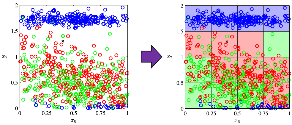
grids respectively in 1, 2, 3 dimensional spaces, the number of the small regions in the grids are respectively 10, 100, 1000. Even though you cannot visualize it anymore, you can make grids for more than 3 dimensional data. If you continue increasing the degree of dimension, the number of grids increases exponentially, and that can soon surpass the number of training data points soon. That means there would be a lot of empty spaces in such high dimensional grids. And the classifying method above: coloring each grid and classifying unknown samples depending on the colors of the grids, does not work out anymore because there would be a lot of empty grids.

* If you are still puzzled by the idea of “more than 3 dimensional grids,” you should not think too much about that now. It is enough if you can get some understandings on high dimensional data after reading the whole article of this.

I said the method above is the most naive way, but other classical classification methods , for example k-nearest neighbors algorithm, are more or less base on a similar idea. Many of classical machine learning algorithms are based on the idea smoothness prior, or local constancy prior. In short in classical ways, you  do not expect data to change so much in a small region, so you can expect unknown samples to be similar to data in vicinity. But that soon turns out to be problematic when the dimension of data is bigger because you will not have training data in vicinity. Plus, in high dimensional data, you cannot necessarily approximate new samples with the data  in vicinity. The ideas of “close,” “nearby,” or “vicinity” get more obscure in high dimensional data. That point is related to the next topic: the intuition have cultivated in normal life is not applicable to higher dimensional data.


2, Bizarre characteristics of high dimensional data

We form our sense of recognition in 3-dimensional way in our normal life. Even though we can visualize only 1, 2, 3 dimensional data, we can actually expand the ideas in 2 or 3 dimensional sense to higher dimensions. For example 4 dimensional cubes, 100 dimensional spheres, or orthogonality in 255 dimensional space. Again, you cannot exactly visualize those ideas, and for many people, such high dimensional phenomenon are just imaginary matters on blackboards.


Those high dimensional ideas are designed to retain some conditions in 1, 2, or 3 dimensional space. Let’s take an example of spheres in several dimensional spaces. One general condition of spheres, or to be exact the surfaces of spheres, are they are a set of points, whose distance from the center point are all the same.

For example you can calculate the value of a D-ball, a sphere with radius r in D dimensional space as below.

Of course when D is bigger than 3, you cannot visualize such sphere anymore, but you define such D-ball if you generalize the some features of sphere to higher dimensional space.

Just in case you are not so familiar with linear algebra, geometry, or the idea of high dimensional space, let’s see what D-ball means concretely.


But there is one severe problem: the behaviors of data in high dimensional field is quite different from those in two or three dimensional space. To be concrete, in high dimensional field, cubes are spiky, you have to move like Pac-Man, and M & M’s Chocolate looks empty inside but tastes normal.


2_1: spiky cubes
Let’s look take an elementary-school-level example of geometry first.


In the first section, I wrote about grids in several dimensions. “Grids” in that case are the same as “hypercubes.” Hypercubes mean generalized grids or cubes in high dimensional space.


* You can confirm that the higher the dimension is the more spiky hypercube becomes, by comparing the volume of the hypercube and the volume of the D-ball inscribed inside the hypercube. Thereby it can be proved that the volume of hypercube concentrates on the corners of the hypercube. Plus, as I mentioned the longest diagonal distance of hypercube gets longer as dimension degree increases. That is why hypercube is said to be spiky. For mathematical proof, please check the Exercise 1.19 of PRML.

2_2: Pac-Man walking

Next intriguing phenomenon in high dimensional field is that most of pairs of vectors in high dimensional space are orthogonal. First of all, let’s see a general meaning of orthogonality of vectors in high dimensional space.

2_3: empty M & M’s chocolate

That is why, in high dimensional space, M & M’s chocolate look empty but tastes normal: all the chocolate are concentrated beneath the sugar coating. Of course this is also contrary to our daily sense, and inside M & M’s chocolate is a mysterious world.


This fact is especially problematic because many machine learning algorithms depends on distances between pairs of data points. Even if you van approximate the distance between two points as zero, like you do in ////, there is no guarantee that you can do the same thing in higher dimensional


3, Peeking phenomenon

Simple RNN

Back propagation of LSTM: just get ready for the most tiresome part

First of all, the summary of this article is “please just download my Power Point slides and be patient, following the equations.” I am not supposed to use so many mathematics when I write articles on Data Science Blog. However using little mathematics when I talk about LSTM backprop is like writing German, never caring about “der,” “die,” “das,” or speaking little English during English classes (, which most high school English teachers in Japan do,) or writing Japanese without using any Chinese characters (, which looks like a terrible handwriting by a drug addict). In short, that is ridiculous.

In this article I will just give you some tips to get ready for the most tiresome part of understanding LSTM.

1, Chain rules

In fact this article is virtually an article on chain rules of differentiation. Even if you have clear understandings on chain rules, I recommend you to take a look at this section. If you have written down all the equations of back propagation of DCL, you would have seen what chain rules are. Even simple chain rules for backprop of normal DCL can be difficult to some people, but when it comes to backprop of LSTM, it is a monster of chain rules. I think using graphical models would help you understand what chain rules are like. Graphical models are basically used to describe the relations  of variables and functions in probabilistic models, so to be exact I am going to use “something like graphical models” in this article. Not that this is a common way to explain chain rules.

First, let’s think about the simplest type of chain rule. Assume that you have a function $f=f(x)=f(x(y))$, and relations of the functions are displayed as the graphical model at the left side of the figure below. Variables are a type of function, so you should think that every node in graphical models denotes a function. Arrows in purple in the right side of the chart show how information propagate in differentiation.

Next, if you a function $f$ , which has two variances  $x_1$ and $x_2$. And both of the variances also share two variances  $y_1$ and $y_2$. When you take partial differentiation of $f$ with respect to $y_1$ or $y_2$, the formula is a little tricky. Let’s think about how to calculate $\frac{\partial f}{\partial y_1}$. The variance $y_1$ propagates to $f$ via $x_1$ and $x_2$. In this case the partial differentiation has two terms as below.

In chain rules, you have to think about all the routes where a variance can propagate through. If you generalize chain rules, that is like below, and you need to understand chain rules in this way to understanding any types of back propagation.

The figure above shows that if you calculate partial differentiation of $f$ with respect to $y_i$, the partial differentiation has $n$ terms in total because $y_i$ propagates to $f$ via $n$ variances.


2, Chain rules in LSTM

I would like you to remember the figure I used to show how errors propagate backward during backprop of simple RNNs. The errors at the last time step propagates only at the last time step.

At RNN block level, the flows of errors are the same in LSTM backprop, but the flow of errors in each block is much more complicated in LSTM backprop.

3, How LSTMs tackle exploding/vanishing gradients problems

LSTMs do not solve, vanishing gradient problems, but instead they mitigate vanishing/exploding gradient problems.

Data Science in Engineering Process - Product Lifecycle Management

How to develop digital products and solutions for industrial environments?

The Data Science and Engineering Process in PLM.

Huge opportunities for digital products are accompanied by huge risks

Digitalization is about to profoundly change the way we live and work. The increasing availability of data combined with growing storage capacities and computing power make it possible to create data-based products, services, and customer specific solutions to create insight with value for the business. Successful implementation requires systematic procedures for managing and analyzing data, but today such procedures are not covered in the PLM processes.

From our experience in industrial settings, organizations start processing the data that happens to be available. This data often does not fully cover the situation of interest, typically has poor quality, and in turn the results of data analysis are misleading. In industrial environments, the reliability and accuracy of results are crucial. Therefore, an enormous responsibility comes with the development of digital products and solutions. Unless there are systematic procedures in place to guide data management and data analysis in the development lifecycle, many promising digital products will not meet expectations.

Various methodologies exist but no comprehensive framework

Over the last decades, various methodologies focusing on specific aspects of how to deal with data were promoted across industries and academia. Examples are Six Sigma, CRISP-DM, JDM standard, DMM model, and KDD process. These methodologies aim at introducing principles for systematic data management and data analysis. Each methodology makes an important contribution to the overall picture of how to deal with data, but none provides a comprehensive framework covering all the necessary tasks and activities for the development of digital products. We should take these approaches as valuable input and integrate their strengths into a comprehensive Data Science and Engineering framework.

In fact, we believe it is time to establish an independent discipline to address the specific challenges of developing digital products, services and customer specific solutions. We need the same kind of professionalism in dealing with data that has been achieved in the established branches of engineering.

Data Science and Engineering as new discipline

Whereas the implementation of software algorithms is adequately guided by software engineering practices, there is currently no established engineering discipline covering the important tasks that focus on the data and how to develop causal models that capture the real world. We believe the development of industrial grade digital products and services requires an additional process area comprising best practices for data management and data analysis. This process area addresses the specific roles, skills, tasks, methods, tools, and management that are needed to succeed.

Figure: Data Science and Engineering as new engineering discipline

More than in other engineering disciplines, the outputs of Data Science and Engineering are created in repetitions of tasks in iterative cycles. The tasks are therefore organized into workflows with distinct objectives that clearly overlap along the phases of the PLM process.

Feasibility of Objectives
  Understand the business situation, confirm the feasibility of the product idea, clarify the data infrastructure needs, and create transparency on opportunities and risks related to the product idea from the data perspective.
Domain Understanding
  Establish an understanding of the causal context of the application domain, identify the influencing factors with impact on the outcomes in the operational scenarios where the digital product or service is going to be used.
Data Management
  Develop the data management strategy, define policies on data lifecycle management, design the specific solution architecture, and validate the technical solution after implementation.
Data Collection
  Define, implement and execute operational procedures for selecting, pre-processing, and transforming data as basis for further analysis. Ensure data quality by performing measurement system analysis and data integrity checks.
Modeling
  Select suitable modeling techniques and create a calibrated prediction model, which includes fitting the parameters or training the model and verifying the accuracy and precision of the prediction model.
Insight Provision
  Incorporate the prediction model into a digital product or solution, provide suitable visualizations to address the information needs, evaluate the accuracy of the prediction results, and establish feedback loops.

Real business value will be generated only if the prediction model at the core of the digital product reliably and accurately reflects the real world, and the results allow to derive not only correct but also helpful conclusions. Now is the time to embrace the unique chances by establishing professionalism in data science and engineering.

Authors

Peter Louis                               

Peter Louis is working at Siemens Advanta Consulting as Senior Key Expert. He has 25 years’ experience in Project Management, Quality Management, Software Engineering, Statistical Process Control, and various process frameworks (Lean, Agile, CMMI). He is an expert on SPC, KPI systems, data analytics, prediction modelling, and Six Sigma Black Belt.


Ralf Russ    

Ralf Russ works as a Principal Key Expert at Siemens Advanta Consulting. He has more than two decades experience rolling out frameworks for development of industrial-grade high quality products, services, and solutions. He is Six Sigma Master Black Belt and passionate about process transparency, optimization, anomaly detection, and prediction modelling using statistics and data analytics.4


Hypothesis Test for real problems

Hypothesis tests are significant for evaluating answers to questions concerning samples of data.

A statistical hypothesis is a belief made about a population parameter. This belief may or might not be right. In other words, hypothesis testing is a proper technique utilized by scientist to support or reject statistical hypotheses. The foremost ideal approach to decide if a statistical hypothesis is correct is examine the whole population.

Since that’s frequently impractical, we normally take a random sample from the population and inspect the equivalent. Within the event sample data set isn’t steady with the statistical hypothesis, the hypothesis is refused.

Types of hypothesis:

There are two sort of hypothesis and both the Null Hypothesis (Ho) and Alternative Hypothesis (Ha) must be totally mutually exclusive events.

• Null hypothesis is usually the hypothesis that the event wont’t happen.

• Alternative hypothesis is a hypothesis that the event will happen.

Why we need Hypothesis Testing?

Suppose a specific cosmetic producing company needs to launch a new Shampoo in the market. For this situation they will follow Hypothesis Testing all together decide the success of new product in the market.

Where likelihood of product being ineffective in market is undertaken as Null Hypothesis and likelihood of product being profitable is undertaken as Alternative Hypothesis. By following the process of Hypothesis testing they will foresee the accomplishment.

How to Calculate Hypothesis Testing?

  • State the two theories with the goal that just one can be correct, to such an extent that the two occasions are totally unrelated.
  • Now figure a study plan, that will lay out how the data will be assessed.
  • Now complete the plan and genuinely investigate the sample dataset.
  • Finally examine the outcome and either accept or reject the null hypothesis.

Another example

Assume, Person have gone after a typing job and he has expressed in the resume that his composing speed is 70 words per minute. The recruiter might need to test his case. On the off chance that he sees his case as adequate, he will enlist him in any case reject him. Thus, he types an example letter and found that his speed is 63 words a minute. Presently, he can settle on whether to employ him or not.  In the event that he meets all other qualification measures. This procedure delineates Hypothesis Testing in layman’s terms.

In statistical terms Hypothesis his typing speed is 70 words per minute is a hypothesis to be tested so-called null hypothesis. Clearly, the alternating hypothesis his composing speed isn’t 70 words per minute.

So, normal composing speed is population parameter and sample composing speed is sample statistics.

The conditions of accepting or rejecting his case is to be chosen by the selection representative. For instance, he may conclude that an error of 6 words is alright to him so he would acknowledge his claim between 64 to 76 words per minute. All things considered, sample speed 63 words per minute will close to reject his case. Furthermore, the choice will be he was producing a fake claim.

In any case, if the selection representative stretches out his acceptance region to positive/negative 7 words that is 63 to 77 words, he would be tolerating his case.

In this way, to finish up, Hypothesis Testing is a procedure to test claims about the population dependent on sample. It is a fascinating reasonable subject with a quite statistical jargon. You have to dive more to get familiar with the details.

Significance Level and Rejection Region for Hypothesis

Type I error probability is normally indicated by α and generally set to 0.05.  The value of α is recognized as the significance level.

The rejection region is the set of sample data that prompts the rejection of the null hypothesis.  The significance level, α, decides the size of the rejection region.  Sample results in the rejection region are labelled statistically significant at level of α .

The impact of differing α is that If α is small, for example, 0.01, the likelihood of a type I error is little, and a ton of sample evidence for the alternative hypothesis is needed before the null hypothesis can be dismissed. Though, when α is bigger, for example, 0.10, the rejection region is bigger, and it is simpler to dismiss the null hypothesis.

Significance from p-values

A subsequent methodology is to evade the utilization of a significance level and rather just report how significant the sample evidence is. This methodology is as of now more widespread.  It is accomplished by method of a p value. P value is gauge of power of the evidence against null hypothesis. It is the likelihood of getting the observed value of test statistic, or value with significantly more prominent proof against null hypothesis (Ho), if the null hypothesis of an investigation question is true. The less significant the p value, the more proof there is supportive of the alternative hypothesis. Sample evidence is measurably noteworthy at the α level just if the p value is less than α. They have an association for two tail tests. When utilizing a confidence interval to playout a two-tailed hypothesis test, reject the null hypothesis if and just if the hypothesized value doesn’t lie inside a confidence interval for the parameter.

Hypothesis Tests and Confidence Intervals

Hypothesis tests and confidence intervals are cut out of the same cloth. An event whose 95% confidence interval reject the hypothesis is an event for which p<0.05 under the relating hypothesis test, and the other way around. A p value is letting you know the greatest confidence interval that despite everything prohibits the hypothesis. As such, if p<0.03 against the null hypothesis, that implies that a 97% confidence interval does exclude the null hypothesis.

Hypothesis Tests for a Population Mean

We do a t test on the ground that the population mean is unknown. The general purpose is to contrast sample mean with some hypothetical population mean, to assess whether the watched the truth is such a great amount of unique in relation to the hypothesis that we can say with assurance that the hypothetical population mean isn’t, indeed, the real population mean.

Hypothesis Tests for a Population Proportion

At the point when you have two unique populations Z test facilitates you to choose if the proportion of certain features is the equivalent or not in the two populations. For instance, if the male proportion is equivalent between two nations.

Hypothesis Test for Equal Population Variances

F Test depends on F distribution and is utilized to think about the variance of the two impartial samples. This is additionally utilized with regards to investigation of variance for making a decision about the significance of more than two sample.

T test and F test are totally two unique things. T test is utilized to evaluate the population parameter, for example, population mean, and is likewise utilized for hypothesis testing for population mean. However, it must be utilized when we don’t know about population standard deviation. On the off chance that we know the population standard deviation, we will utilize Z test. We can likewise utilize T statistic to approximate population mean. T statistic is likewise utilised for discovering the distinction in two population mean with the assistance of sample means.

Z statistic or T statistic is utilized to assess population parameters such as population mean and population proportion. It is likewise used for testing hypothesis for population mean and population proportion. In contrast to Z statistic or T statistic, where we manage mean and proportion, Chi Square or F test is utilized for seeing if there is any variance inside the samples. F test is the proportion of fluctuation of two samples.

Conclusion

Hypothesis encourages us to make coherent determinations, the connection among variables, and gives the course to additionally investigate. Hypothesis for the most part results from speculation concerning studied behaviour, natural phenomenon, or proven theory. An honest hypothesis ought to be clear, detailed, and reliable with the data. In the wake of building up the hypothesis, the following stage is validating or testing the hypothesis. Testing of hypothesis includes the process that empowers to concur or differ with the expressed hypothesis.

AI Voice Assistants are the Next Revolution: How Prepared are You?

By 2022, voice-based shopping is predicted to rise to USD 40 billion, based on the data from OC&C Strategy Consultants. We’re in an era of ‘voice’ where drastic transformation is seen between the way AI and voice recognition are changing the way we live.

According to the survey, the surge of voice assistants is said to be driven by the number of homes that used smart speakers, as such that the rise is seen to grow from 13% to 55%. Nonetheless, Amazon will be one of the leaders to dominate the new channel having the largest market share.

Perhaps this is the first time you’ve heard about the voice revolution. Well, why not, based on multiple researchers, it is estimated that the number of voice assistants will grow to USD 8 billion by 2023 from USD 2.5 billion in 2018.

But what is voice revolution or voice assistant or voice search?

It was only until recently that the consumers have started learning about voice assistants which further predicts to exist in the future.

You’ve heard of Alexa, Cortana, Siri, and Google Assistant, these technologies are some of the world’s greatest examples of voice assistants. They will further help to drive consumer behavior as well as prepare the companies and adjust based on the industry demands. Consumers can now transform the way they act, search, and advertise their brand through voice technology.

Voice search is a technology to help users or consumers perform a search on the website by simply asking a question on their smartphone, their computer, or their smart device.

The voice assistant awareness: Why now?

As surveyed by PwC, amongst the 90% respondents, about 72% have been recorded to use voice assistant while merely 10% said they were clueless about voice-enabled devices and products. It is noted, the adoption of voice-enabled was majorly driven by children, young consumers, and households earning an income of around >USD100k.

Let us have a glance to ensure the devices that are used mainly for voice assistance: –

  • Smartphone – 57%
  • Desktop – 29%
  • Tablet – 29%
  • Laptop – 29%
  • Speaker – 27%
  • TV remote – 21%
  • Car navigation – 20%
  • Wearable – 14%

According to the survey, most consumers that use voice-assistants were the younger generation, aged between 18-24.

While individuals between the ages 25-49 were said to use these technologies in a much more statistical manner, and are called the “heavy users.”

Significance of mobile voice assistants: What is the need?

Although mobile is accessible everywhere, you will merely find three out of four consumers using mobile voice assistants in their household i.e. 74%.

Mobile-based AI chatbots have taken our lives by storm, thus providing the best solution to both the customers and agents in varied areas – insurance, travel, and education, etc.

A certain group of individuals said they needed privacy while speaking to their device and that sending a voice command in public is weird.

Well, this simply explains why 18-24 aged group individuals prefer less use of voice assistants. However, this age group tends to spend more time out of their homes.

Situations where voice assistants can be used – standalone speakers Vs mobile

Cooking

  • Standalone speakers – 65%
  • Mobile – 37%

Multitasking

  • Standalone speakers – 62%
  • Mobile – 12%

Watching TV

  • Standalone speakers – 57%
  • Mobile – 43%

In bed

  • Standalone speakers – 38%
  • Mobile – 37%

Working

  • Standalone speakers – 29%
  • Mobile – 25%

Driving

  • Standalone speakers – 0%
  • Mobile – 40%

By the end of 2020, nearly half of all the searches made will be voice-based, as predicted by Comscore, a media analytics firm.

Don’t you think voice-based assistant is changing the way businesses function? Thanks to the advent of AI!

  • A 2018 study on AI chatbots and voice assistants by Spiceworks said, 24% of businesses that were spread largely, and 16% of smaller businesses have already started using AI technologies in their workplaces. While 25% of the business market is expected to adopt AI within the next 12 months.

Surprisingly, voice-based assistants such as Siri, Google Assistant, and Cortana are some of the most prominent technologies these businesses are using in their workstations.

Where will the next AI voice revolution take us?

Voice-authorized transactions

Paypal, an online payment gateway now leverages Siri and Alexa’s voice recognition capability, thus, allowing users to make payments, check their balance, and ask payments from people via voice command.

Voice remote control – AI-powered

Communications conglomerate Comcast, an American telecommunications and media conglomerate introduces their first-ever X1 voice remote control that provides both natural image processing and voice recognition.

With the help of deep learning, the X1 can easily come up with better search results with just a press of the button telling what your television needs to do next.

Voice AI-enabled memos and analytics

Salesforce recently unveiled Einstein Voice which is an AI assistant that helps in entering critical data the moment it hears, making use of the voice command. This AI assistant also initiates in interpreting voice memos. Besides this, the voice bots accompanying Einstein Voice also helps the company create their customized voice bots to answer customer queries.

Voice-activated ordering

It is astonishing to see how Domino’s is using voice-activated feature automate orders made over the phone by customers. Well, welcome to the era of voice revolution.

This app, developed by Nuance Communications already has a Siri like voice recognition feature that allows customers to place their orders just like how they would be doing it in front of the cash counter making your order to take place efficiently.

As more businesses look forward to breaking down the roadblocks between a consumer and a brand, voice search now projects to become an impactful technology of bridging the gap.

Simple RNN

A gentle introduction to the tiresome part of understanding RNN

Just as a normal conversation in a random pub or bar in Berlin, people often ask me “Which language do you use?” I always answer “LaTeX and PowerPoint.”

I have been doing an internship at DATANOMIQ and trying to make straightforward but precise study materials on deep learning. I myself started learning machine learning in April of 2019, and I have been self-studying during this one-year-vacation of mine in Berlin.

Many study materials give good explanations on densely connected layers or convolutional neural networks (CNNs). But when it comes to back propagation of CNN and recurrent neural networks (RNNs), I think there’s much room for improvement to make the topic understandable to learners.

Many study materials avoid the points I want to understand, and that was as frustrating to me as listening to answers to questions in the Japanese Diet, or listening to speeches from the current Japanese minister of the environment. With the slightest common sense, you would always get the feeling “How?” after reading an RNN chapter in any book.

This blog series focuses on the introductory level of recurrent neural networks. By “introductory”, I mean prerequisites for a better and more mathematical understanding of RNN algorithms.

I am going to keep these posts as visual as possible, avoiding equations, but I am also going to attach some links to check more precise mathematical explanations.

This blog series is composed of five contents.:

  1. Prerequisites for understanding RNN at a more mathematical level
  2. Simple RNN: the first foothold for understanding LSTM
  3. A brief history of neural nets: everything you should know before learning LSTM
  4. LSTM and its forward propagation (to be published soon)
  5. LSTM and Its back propagation (to be published soon)


Business Data is changing the world’s view towards Green Energy

Energy conservation is one of the main stressed points all around the globe. In the past 30 years, researches in the field of energy conservation and especially green energy have risen to another level. The positive outcomes of these researches have given us a gamut of technologies that can aid in preserving and utilize green energy. It has also reduced the over-dependency of companies on fossil fuels such as oil, coal, and natural gas.

Business data and analytics have all the power and the potential to take the business organizations forward in the future and conquer new frontiers. Seizing the opportunities presented by Green energy, market leaders such as Intel and Google have already implemented it, and now they enjoy the rich benefits of green energy sources.

Business data enables the organizations to keep an eye on measuring the positive outcomes by adopting the green energies. According to a report done by the World energy outlook, the global wind energy capacity will increase by 85% by the year 2020, reaching 1400 TWh. Moreover, in the Paris Summit, more than 170 countries around the world agreed on reducing the impact of global warming by harnessing energy from green energy sources. And for this to work, Big Data Analytics will play a pivotal role.

Overview of Green energy

In simpler terms, Green Energy is the energy coming from natural sources such as wind, sun, plants, tides, and geothermal heat. In contrast to fossil fuels, green energy resources can be replenished in a short period, and one can use them for longer periods. Green energy sources have a minimal ill effect on the environment as compared to fossil fuels. In addition to this, fossil fuels can be replaced by green energy sources in many areas like providing electricity, fuel for motor vehicles, etc..

With the help of business data, organizations throughout the world can change the view of green energy. Big Data can show how different types of green energy sources can help businesses and accelerate sustainable expansion.

Below are the different types of green energy sources:

  • Wind Power
  • Solar Power
  • Geothermal Energy
  • Hydropower
  • Biofuels
  • Bio-mass

Now we present before you a list of advantages that green energy or renewable energy sources have brought to the new age businesses.

Profits on the rise

If the energy produced is more than the energy used, the organizations can sell it back to the grids and earn profit out of it. Green energy sources are renewable sources of energy, and with precise data, the companies will get an overall estimation of the requirement of energy.

With Big Data, the organizations can know the history of the demographical location before setting up the factory. For example, if your company is planning to setup a factory in the coastal region, tidal and wind energy would be more beneficial as compared to solar power. Business data will give the complete analysis of the flow of the wind so that the companies can ascertain the best location of the windmill; this will allow them to store the energy in advance and use it as per their requirement. It not only saves money but also provides an extra source of income to the companies. With green energy sources, the production in the company can increase to an unprecedented level and have sustainable growth over the years.

Synchronizing the maintenance process

If there is a rapid inflow of solar and wind energy sources, the amount of power produced will be huge. Many solar panels and windmills are operating in a solar power plant or in a wind energy source, and with many types of equipment, it becomestoo complex to manage. Big Data analytics will assist the companies in streamlining all the operations to a large extent for their everyday work without any hassle.

Moreover, the analytics tool will convey the performance of renewable energy sources under different weather conditions. Thus, the companies will get the perfect idea about the performance of the green energy sources, thus enabling them to take necessary actions as and when required.

Lowering the attrition rate

Researchers have found that more number of employees want to be associated with companies that support green energies. By opting for green energy sources and investing in them, companies are indirectly investing in keeping the workforce intact and lowering the attrition rate. Stats also show the same track as nearly 50% of the working professionals, and almost 2/3rd of the millennial population want to be associated with the companies who are opting for the green energy sources and have a positive impact on environmental conservation.

The employees will not only wish to stay with the organizations for a long time but will also work hard for the betterment of the organization. Therefore, you can concentrate on expanding the business rather than thinking about the replacement of the employees.

Lowering the risk due to Power Outage

The Business Data Analytics will continuously keep updating the requirements of power needed to run the company. Thus the organizations can cut down the risk of the power outage and also the expenses related to it. The companies will know when to halt the energy transmission as they would know if the grid is under some strain or not.

Business analytics and green energy provide a planned power outage to the companies, which is cost-efficient and thus can decrease the product development cost.  Apart from this, companies can store energy for later usage. Practicing this process will help save a lot of money in the long run, proving that investment in green energy sources is a smart investment.

Reducing the maintenance cost

An increasing number of organizations are using renewable sources of energy as it plays a vital role in decreasing production and maintenance costs. The predictive analysis technology helps renewable energy sources to produce more energy at less cost, thus reducing the cost of infrastructure.

Moreover, data analytics will make green energy sources more bankable for companies. As organizations will have a concrete amount of data related to the energy sources, they can use it wisely on a more productive basis

Escalating Energy Storage

Green energy sources can be stored in bulk and used as per requirement by the business organizations. Using green energy on a larger basis will even allow companies to completely get rid of fossil fuels and thus work towards the betterment of the environment. Big Data analytics with AI and cloud-enabled systems help organizations store renewable energies such as Wind and Solar.

Moreover, it gathers information for the businesses and gives the complete analysis of the exact amount of energy required to complete a particular task. The data will also automate cost savings as it can predict the client’s needs. Based on business data, companies can store renewable energy sources in a better manner.

With Business data analytics, the companies can store energy when it is cheap and use it according to the needs when the energy rates go higher. Although predicting the requirement of storage is a complicated process, with Artificial Intelligence (AI) at work, you can analyze the data efficiently.

Bundling Up

Green energy sources will play a pivotal role in deciding the future of the businesses as fossil fuels are available in a certain limit. Moreover, astute business data analysts will assist the organizations to not only use renewable energy sources in a better manner but also to form a formidable workforce. The data support in the green energy sector will also provide sustainable growth to the companies, monitor their efforts, and assist them in the long run.

Predictive Analytics World 2020 Healthcare

Difficult times call for creative measures

Predictive Analytics World for Healthcare will go virtual and you still have time to join us!

What do you have in store for me?

We will provide a live-streamed virtual version of healthcare Munich 2020 on 11-12 May, 2020: you will be able to attend sessions and to interact and connect with the speakers and fellow members of the data science community including sponsors and exhibitors from your home or your office.

What about the workshops?

The workshops will also be held virtually on the planned date:
13 May, 2020.

Get a complimentary virtual sneak preview!

If you would like to join us for a virtual sneak preview of the workshop „Data Thinking“ on Thursday, April 16, so you can familiarise yourself with the quality of the virtual edition of both conference and workshops and how the interaction with speakers and attendees works, please send a request to registration@risingmedia.com.

Don’t have a ticket yet?

It‘s not too late to join the data science community.
Register by 10 May to receive access to the livestream and recordings.

REGISTER HERE

We’re looking forward to see you – virtually!

This year Predictive Analytics World for Healthcare runs alongside Deep Learning World and Predictive Analytics World for Industry 4.0.

Customer Journey Mapping: The data-driven approach to understanding your users

Businesses across the globe are on a mission to know their customers inside out – something commonly referred to as customer-centricity. It’s an attempt to better understand the needs and wants of customers in order to provide them with a better overall experience.

But while this sounds promising in theory, it’s much harder to achieve in practice. To really know your customer you must not only understand what they want, but you also need to hone in on how they want it, when they want it and how often as well.

In essence, your business should use customer journey mapping. It allows you to visualise customer feelings and behaviours through the different stages of their journey – from the first interaction, right up until the point of purchase and beyond.

The Data-Driven Approach 

To ensure your customer journey mapping is successful, you must conduct some extensive research on your customers. You can’t afford to make decisions based on feelings and emotions alone. There are two types of research that you should use for customer journey mapping – quantitative and qualitative research.

Quantitative data is best for analysing the behaviour of your customers as it identifies their habits over time. It’s also extremely useful for confirming any hypotheses you may have developed. That being so, relying solely upon quantitative data can present one major issue – it doesn’t provide you with the specific reason behind those behaviours.

That’s where qualitative data comes to the rescue. Through data collection methods like surveys, interviews and focus groups, you can figure out the reasoning behind some of your quantitative data trends. The obvious downside to qualitative data is its lack of evidence and its tendency to be subjective. Therefore, a combination of both quantitative and qualitative research is most effective.

Creating A Customer Persona

A customer persona is designed to help businesses understand the key traits of specific groups of people. For example, those defined by their age range or geographic location. A customer persona can help improve your customer journey map by providing more insight into the behavioural trends of your “ideal” customer. 

The one downside to using customer personas is that they can be over-generalised at times. Just because a group of people shares a similar age, for example, it does not mean they all share the same beliefs and interests. Nevertheless, creating a customer persona is still beneficial to customer journey mapping – especially if used in combination with the correct customer journey analytics tools.

All Roads Lead To Customer-centricity 

To achieve customer-centricity, businesses must consider using a data-driven approach to customer journey mapping. First, it requires that you achieve a balance between both quantitative and qualitative research. Quantitative research will provide you with definitive trends while qualitative data gives you the reasoning behind those trends. 

To further increase the effectiveness of your customer journey map, consider creating customer personas. They will give you further insight into the behavioural trends within specific groups. 

This article was written by TAP London. Experts in the Adobe Experience Cloud, TAP London help brands organise data to provide meaningful insight and memorable customer experiences. Find out more at wearetaplondon.com.