Illustrative introductions on dimension reduction

“What is your image on dimensions?”
….That might be a cheesy question to ask to reader of Data Science Blog, but most people, with no scientific background, would answer “One dimension is a line, and two dimension is a plain, and we live in three-dimensional world.” After that if you ask “How about the fourth dimension?” many people would answer “Time?”

Terms like “multi dimensional something” is often used in science fictions because it’s a convenient black box when you make a fantasy story, and I’m sure many authors would not have thought that much about what those dimensions are.

In Japanese, if you say “He likes two dimension.” that means he prefers anime characters to real women, as is often the case with Japanese computer science students.

The meanings of “dimensions” depend on the context, but in data science dimension is in short the number of rows of your Excel data.

When you study data science or machine learning, usually you should start with understanding the algorithms with 2 or 3 dimensional data, and you can apply those ideas to any D dimensional data.
But of course you cannot visualize D dimensional data anymore, and that is almost an imaginary world on blackboards.

In this blog series I am going to explain algorithms for dimension reductions, such as PCA, LDA, and t-SNE, with 2 or 3 dimensional visible data. Along with that, I am going to delve into the meaning of calculations so that you can understand them in more like everyday-life sense.

This article series is going to be roughly divided into the contents below.

  1. Curse of Dimensionality (to be published soon)
  2. PCA, LDA (to be published soon)
  3. Rethinking eigen vectors (to be published soon)
  4. KL expansion and subspace method (to be published soon)
  5. Autoencoder as dimension reduction (to be published soon)
  6. t-SNE (to be published soon)

I hope you could see that reducing dimension is one of the fundamental approaches in data science or machine learning.

Spiky cubes, Pac-Man walking, empty M&M’s chocolate: curse of dimensionality

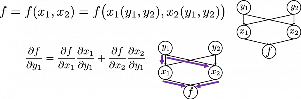
“Curse of dimensionality” means the difficulties of machine learning which arise when the dimension of data is higher. In short if the data have too many features like “weight,” “height,” “width,” “strength,” “temperature”…. that can undermine the performances of machine learning. The fact might be contrary to your image which you get from the terms “big” data or “deep” learning. You might assume that the more hints you have, the better the performances of machine learning are. There are some reasons for curse of dimensionality, and in this article I am going to introduce three major reasons below.

  1. High dimensional data usually have rich expressiveness, but usually training data are too poor for that.
  2. The behaviors of data points in high dimensional space are totally different from our common sense.
  3. More irrelevant featreus lead to confusions in recognition or decision making.

Through these topics, you will see that you always have to think about which features to use considering the number of data points.

1, Number of samples and degree of dimension

The most straightforward demerit of adding many features, or increasing dimensions of data, is the growth of computational costs. More importantly, however, you always have to think about the degree of dimensions in relation of the number of data points you have. Let me take a simple example in a book “Pattern Recognition and Machine Learning” by C. M. Bishop (PRML). This is an example of measurements of a pipeline. The figure below shows a comparison plot of 3 classes (red, green and blue), with parameter x7 plotted against parameter x6 out of 12 parameters.

* The meaning of data is not important in this article. If you are interested please refer to the appendix in PRML.

Assume that we are interested in classifying the cross in black into one of the three classes. One of the most naive ideas of this classification is dividing the graph into grids and labeling each grid depending on the number of samples in the classes (which are colored at the right side of the figure). And you can classify the test sample, the cross in black, into the class of the grid where the test sample is in.


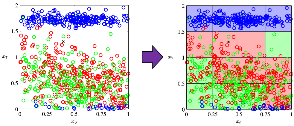
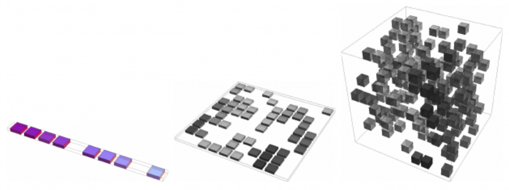
As I mentioned the figure above only two features out of 12 features in total. When the the total number of plots is fixed, and you add remaining ten axes one after another, what would happen? Let’s see what “adding axes” mean. If you are talking about 1, 2, or 3 dimensional grids, you can visualize them. And as you can see from the figure below, if you make each 10^1, 10^2, 100^3 grids respectively in 1, 2, 3 dimensional spaces, the number of the small regions in the grids are respectively 10, 100, 1000. Even though you cannot visualize it anymore, you can make grids for more than 3 dimensional data. If you continue increasing the degree of dimension, the number of grids increases exponentially, and that can soon surpass the number of training data points soon. That means there would be a lot of empty spaces in such high dimensional grids. And the classifying method above: coloring each grid and classifying unknown samples depending on the colors of the grids, does not work out anymore because there would be a lot of empty grids.

* If you are still puzzled by the idea of “more than 3 dimensional grids,” you should not think too much about that now. It is enough if you can get some understandings on high dimensional data after reading the whole article of this.

I said the method above is the most naive way, but other classical classification methods , for example k-nearest neighbors algorithm, are more or less base on a similar idea. Many of classical machine learning algorithms are based on the idea smoothness prior, or local constancy prior. In short in classical ways, you  do not expect data to change so much in a small region, so you can expect unknown samples to be similar to data in vicinity. But that soon turns out to be problematic when the dimension of data is bigger because you will not have training data in vicinity. Plus, in high dimensional data, you cannot necessarily approximate new samples with the data  in vicinity. The ideas of “close,” “nearby,” or “vicinity” get more obscure in high dimensional data. That point is related to the next topic: the intuition have cultivated in normal life is not applicable to higher dimensional data.


2, Bizarre characteristics of high dimensional data

We form our sense of recognition in 3-dimensional way in our normal life. Even though we can visualize only 1, 2, 3 dimensional data, we can actually expand the ideas in 2 or 3 dimensional sense to higher dimensions. For example 4 dimensional cubes, 100 dimensional spheres, or orthogonality in 255 dimensional space. Again, you cannot exactly visualize those ideas, and for many people, such high dimensional phenomenon are just imaginary matters on blackboards.


Those high dimensional ideas are designed to retain some conditions in 1, 2, or 3 dimensional space. Let’s take an example of spheres in several dimensional spaces. One general condition of spheres, or to be exact the surfaces of spheres, are they are a set of points, whose distance from the center point are all the same.

For example you can calculate the value of a D-ball, a sphere with radius r in D dimensional space as below.

Of course when D is bigger than 3, you cannot visualize such sphere anymore, but you define such D-ball if you generalize the some features of sphere to higher dimensional space.

Just in case you are not so familiar with linear algebra, geometry, or the idea of high dimensional space, let’s see what D-ball means concretely.


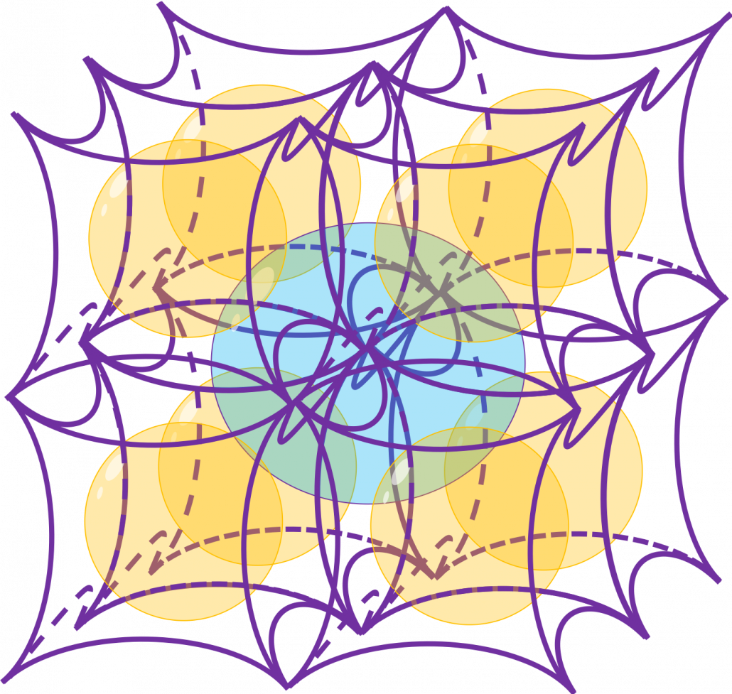
But there is one severe problem: the behaviors of data in high dimensional field is quite different from those in two or three dimensional space. To be concrete, in high dimensional field, cubes are spiky, you have to move like Pac-Man, and M & M’s Chocolate looks empty inside but tastes normal.


2_1: spiky cubes
Let’s look take an elementary-school-level example of geometry first.


In the first section, I wrote about grids in several dimensions. “Grids” in that case are the same as “hypercubes.” Hypercubes mean generalized grids or cubes in high dimensional space.


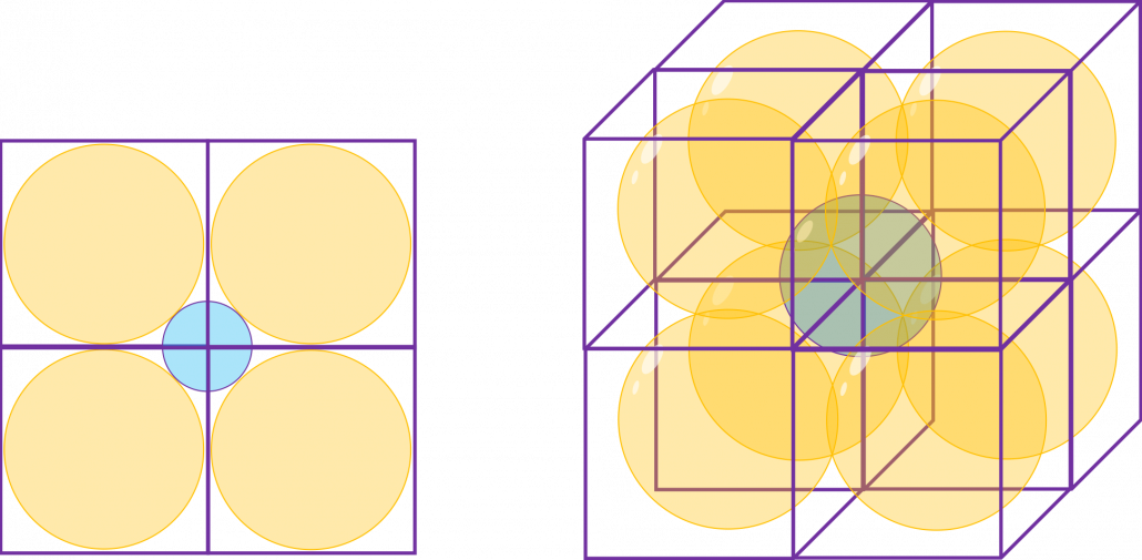
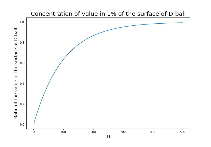
* You can confirm that the higher the dimension is the more spiky hypercube becomes, by comparing the volume of the hypercube and the volume of the D-ball inscribed inside the hypercube. Thereby it can be proved that the volume of hypercube concentrates on the corners of the hypercube. Plus, as I mentioned the longest diagonal distance of hypercube gets longer as dimension degree increases. That is why hypercube is said to be spiky. For mathematical proof, please check the Exercise 1.19 of PRML.

2_2: Pac-Man walking

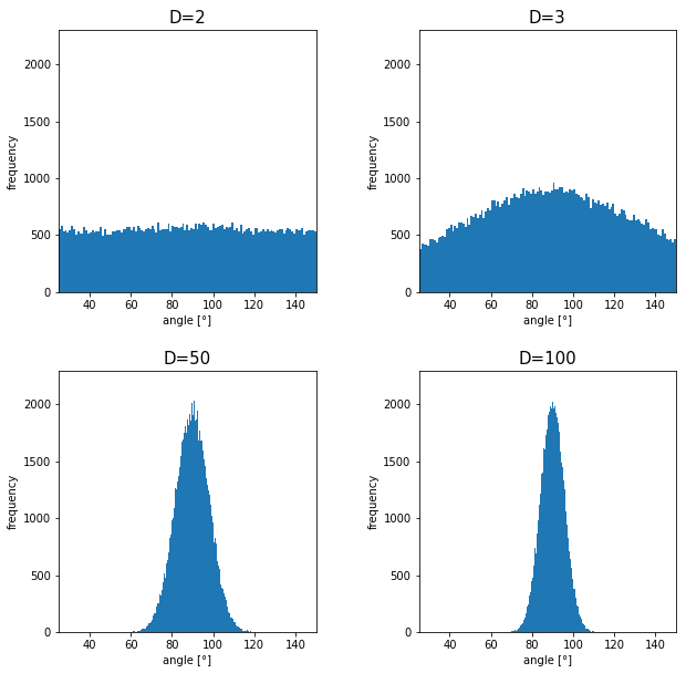
Next intriguing phenomenon in high dimensional field is that most of pairs of vectors in high dimensional space are orthogonal. First of all, let’s see a general meaning of orthogonality of vectors in high dimensional space.

2_3: empty M & M’s chocolate

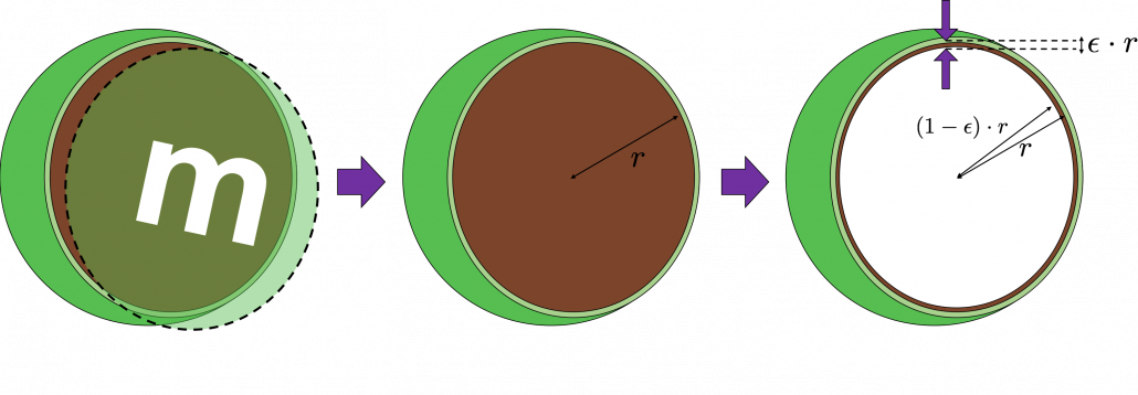
That is why, in high dimensional space, M & M’s chocolate look empty but tastes normal: all the chocolate are concentrated beneath the sugar coating. Of course this is also contrary to our daily sense, and inside M & M’s chocolate is a mysterious world.


This fact is especially problematic because many machine learning algorithms depends on distances between pairs of data points. Even if you van approximate the distance between two points as zero, like you do in ////, there is no guarantee that you can do the same thing in higher dimensional


3, Peeking phenomenon

Simple RNN

Back propagation of LSTM: just get ready for the most tiresome part

First of all, the summary of this article is “please just download my Power Point slides and be patient, following the equations.” I am not supposed to use so many mathematics when I write articles on Data Science Blog. However using little mathematics when I talk about LSTM backprop is like writing German, never caring about “der,” “die,” “das,” or speaking little English during English classes (, which most high school English teachers in Japan do,) or writing Japanese without using any Chinese characters (, which looks like a terrible handwriting by a drug addict). In short, that is ridiculous.

In this article I will just give you some tips to get ready for the most tiresome part of understanding LSTM.

1, Chain rules

In fact this article is virtually an article on chain rules of differentiation. Even if you have clear understandings on chain rules, I recommend you to take a look at this section. If you have written down all the equations of back propagation of DCL, you would have seen what chain rules are. Even simple chain rules for backprop of normal DCL can be difficult to some people, but when it comes to backprop of LSTM, it is a monster of chain rules. I think using graphical models would help you understand what chain rules are like. Graphical models are basically used to describe the relations  of variables and functions in probabilistic models, so to be exact I am going to use “something like graphical models” in this article. Not that this is a common way to explain chain rules.

First, let’s think about the simplest type of chain rule. Assume that you have a function $f=f(x)=f(x(y))$, and relations of the functions are displayed as the graphical model at the left side of the figure below. Variables are a type of function, so you should think that every node in graphical models denotes a function. Arrows in purple in the right side of the chart show how information propagate in differentiation.

Next, if you a function $f$ , which has two variances  $x_1$ and $x_2$. And both of the variances also share two variances  $y_1$ and $y_2$. When you take partial differentiation of $f$ with respect to $y_1$ or $y_2$, the formula is a little tricky. Let’s think about how to calculate $\frac{\partial f}{\partial y_1}$. The variance $y_1$ propagates to $f$ via $x_1$ and $x_2$. In this case the partial differentiation has two terms as below.

In chain rules, you have to think about all the routes where a variance can propagate through. If you generalize chain rules, that is like below, and you need to understand chain rules in this way to understanding any types of back propagation.

The figure above shows that if you calculate partial differentiation of $f$ with respect to $y_i$, the partial differentiation has $n$ terms in total because $y_i$ propagates to $f$ via $n$ variances.


2, Chain rules in LSTM

I would like you to remember the figure I used to show how errors propagate backward during backprop of simple RNNs. The errors at the last time step propagates only at the last time step.

At RNN block level, the flows of errors are the same in LSTM backprop, but the flow of errors in each block is much more complicated in LSTM backprop.

3, How LSTMs tackle exploding/vanishing gradients problems

LSTMs do not solve, vanishing gradient problems, but instead they mitigate vanishing/exploding gradient problems.

Data Science in Engineering Process - Product Lifecycle Management

How to develop digital products and solutions for industrial environments?

The Data Science and Engineering Process in PLM.

Huge opportunities for digital products are accompanied by huge risks

Digitalization is about to profoundly change the way we live and work. The increasing availability of data combined with growing storage capacities and computing power make it possible to create data-based products, services, and customer specific solutions to create insight with value for the business. Successful implementation requires systematic procedures for managing and analyzing data, but today such procedures are not covered in the PLM processes.

From our experience in industrial settings, organizations start processing the data that happens to be available. This data often does not fully cover the situation of interest, typically has poor quality, and in turn the results of data analysis are misleading. In industrial environments, the reliability and accuracy of results are crucial. Therefore, an enormous responsibility comes with the development of digital products and solutions. Unless there are systematic procedures in place to guide data management and data analysis in the development lifecycle, many promising digital products will not meet expectations.

Various methodologies exist but no comprehensive framework

Over the last decades, various methodologies focusing on specific aspects of how to deal with data were promoted across industries and academia. Examples are Six Sigma, CRISP-DM, JDM standard, DMM model, and KDD process. These methodologies aim at introducing principles for systematic data management and data analysis. Each methodology makes an important contribution to the overall picture of how to deal with data, but none provides a comprehensive framework covering all the necessary tasks and activities for the development of digital products. We should take these approaches as valuable input and integrate their strengths into a comprehensive Data Science and Engineering framework.

In fact, we believe it is time to establish an independent discipline to address the specific challenges of developing digital products, services and customer specific solutions. We need the same kind of professionalism in dealing with data that has been achieved in the established branches of engineering.

Data Science and Engineering as new discipline

Whereas the implementation of software algorithms is adequately guided by software engineering practices, there is currently no established engineering discipline covering the important tasks that focus on the data and how to develop causal models that capture the real world. We believe the development of industrial grade digital products and services requires an additional process area comprising best practices for data management and data analysis. This process area addresses the specific roles, skills, tasks, methods, tools, and management that are needed to succeed.

Figure: Data Science and Engineering as new engineering discipline

More than in other engineering disciplines, the outputs of Data Science and Engineering are created in repetitions of tasks in iterative cycles. The tasks are therefore organized into workflows with distinct objectives that clearly overlap along the phases of the PLM process.

Feasibility of Objectives
  Understand the business situation, confirm the feasibility of the product idea, clarify the data infrastructure needs, and create transparency on opportunities and risks related to the product idea from the data perspective.
Domain Understanding
  Establish an understanding of the causal context of the application domain, identify the influencing factors with impact on the outcomes in the operational scenarios where the digital product or service is going to be used.
Data Management
  Develop the data management strategy, define policies on data lifecycle management, design the specific solution architecture, and validate the technical solution after implementation.
Data Collection
  Define, implement and execute operational procedures for selecting, pre-processing, and transforming data as basis for further analysis. Ensure data quality by performing measurement system analysis and data integrity checks.
Modeling
  Select suitable modeling techniques and create a calibrated prediction model, which includes fitting the parameters or training the model and verifying the accuracy and precision of the prediction model.
Insight Provision
  Incorporate the prediction model into a digital product or solution, provide suitable visualizations to address the information needs, evaluate the accuracy of the prediction results, and establish feedback loops.

Real business value will be generated only if the prediction model at the core of the digital product reliably and accurately reflects the real world, and the results allow to derive not only correct but also helpful conclusions. Now is the time to embrace the unique chances by establishing professionalism in data science and engineering.

Authors

Peter Louis                               

Peter Louis is working at Siemens Advanta Consulting as Senior Key Expert. He has 25 years’ experience in Project Management, Quality Management, Software Engineering, Statistical Process Control, and various process frameworks (Lean, Agile, CMMI). He is an expert on SPC, KPI systems, data analytics, prediction modelling, and Six Sigma Black Belt.


Ralf Russ    

Ralf Russ works as a Principal Key Expert at Siemens Advanta Consulting. He has more than two decades experience rolling out frameworks for development of industrial-grade high quality products, services, and solutions. He is Six Sigma Master Black Belt and passionate about process transparency, optimization, anomaly detection, and prediction modelling using statistics and data analytics.4