Data Science für Smart Home im familiengeführten Unternehmen Miele
 Dr. Florian Nielsen ist Principal for AI und Data Science bei Miele im Bereich Smart Home und zuständig für die Entwicklung daten-getriebener digitaler Produkte und Produkterweiterungen. Der studierte Informatiker promovierte an der Universität Ulm zum Thema multimodale kognitive technische Systeme.
Data Science Blog: Herr Dr. Nielsen, viele Unternehmen und Anwender reden heute schon von Smart Home, haben jedoch eher ein Remote Home. Wie machen Sie daraus tatsächlich ein Smart Home?
Tatsächlich entspricht das auch meiner Wahrnehmung. Die bloße Steuerung vernetzter Produkte über digitale Endgeräte macht aus einem vernetzten Produkt nicht gleich ein „smartes“. Allerdings ist diese Remotefunktion ein notwendiges Puzzlestück in der Entwicklung von einem nicht vernetzten Produkt, über ein intelligentes, vernetztes Produkt hin zu einem Ökosystem von sich ergänzenden smarten Produkten und Services. Vernetzte Produkte, selbst wenn sie nur aus der Ferne gesteuert werden können, erzeugen Daten und ermöglichen uns die Personalisierung, Optimierung oder gar Automatisierung von Produktfunktionen basierend auf diesen Daten voran zu treiben. „Smart“ wird für mich ein Produkt, wenn es sich beispielsweise besser den Bedürfnissen des Nutzers anpasst oder über Assistenzfunktionen eine Arbeitserleichterung im Alltag bietet.
Data Science Blog: Smart Home wiederum ist ein großer Begriff, der weit mehr als Geräte für Küchen und Badezimmer betrifft. Wie weit werden Sie hier ins Smart Home vordringen können?
Smart Home ist für mich schon fast ein verbrannter Begriff. Der Nutzer assoziiert hiermit doch vor allem die Steuerung von Heizung und Rollladen. Im Prinzip geht es doch um eine Vision in der sich smarte, vernetzte Produkt in ein kontextbasiertes Ökosystem einbetten um den jeweiligen Nutzer in seinem Alltag, nicht nur in seinem Zuhause, Mehrwert mit intelligenten Produkten und Services zu bieten. Für uns fängt das beispielsweise nicht erst beim Starten des Kochprozesses mit Miele-Geräten an, sondern deckt potenziell die komplette „User Journey“ rund um Ernährung (z. B. Inspiration, Einkaufen, Vorratshaltung) und Kochen ab. Natürlich überlegen wir verstärkt, wie Produkte und Services unser existierendes Produktportfolio ergänzen bzw. dem Nutzer zugänglicher machen könnten, beschränken uns aber hierauf nicht. Ein zusätzlicher für uns als Miele essenzieller Aspekt ist allerdings auch die Privatsphäre des Kunden. Bei der Bewertung potenzieller Use-Cases spielt die Privatsphäre unserer Kunden immer eine wichtige Rolle.
Data Science Blog: Die meisten Data-Science-Abteilungen befassen sich eher mit Prozessen, z. B. der Qualitätsüberwachung oder Prozessoptimierung in der Produktion. Sie jedoch nutzen Data Science als Komponente für Produkte. Was gibt es dabei zu beachten?
Kundenbedürfnisse. Wir glauben an nutzerorientierte Produktentwicklung und dementsprechend fängt alles bei uns bei der Identifikation von Bedürfnissen und potenziellen Lösungen hierfür an. Meist starten wir mit „Design Thinking“ um die Themen zu identifizieren, die für den Kunden einen echten Mehrwert bieten. Wenn dann noch Data Science Teil der abgeleiteten Lösung ist, kommen wir verstärkt ins Spiel. Eine wesentliche Herausforderung ist, dass wir oft nicht auf der grünen Wiese starten können. Zumindest wenn es um ein zusätzliches Produktfeature geht, das mit bestehender Gerätehardware, Vernetzungsarchitektur und der daraus resultierenden Datengrundlage zurechtkommen muss. Zwar sind unsere neuen Produktgenerationen „Remote Update“-fähig, aber auch das hilft uns manchmal nur bedingt. Dementsprechend ist die Antizipation von Geräteanforderungen essenziell. Etwas besser sieht es natürlich bei Umsetzungen von cloud-basierten Use-Cases aus.
Data Science Blog: Es heißt häufig, dass Data Scientists kaum zu finden sind. Ist Recruiting für Sie tatsächlich noch ein Thema?
Data Scientists, hier mal nicht interpretiert als Mythos „Unicorn“ oder „Full-Stack“ sind natürlich wichtig, und auch nicht leicht zu bekommen in einer Region wie Gütersloh. Aber Engineers, egal ob Data, ML, Cloud oder Software generell, sind der viel wesentlichere Baustein für uns. Für die Umsetzung von Ideen braucht es nun mal viel Engineering. Es ist mittlerweile hinlänglich bekannt, dass Data Science einen zwar sehr wichtigen, aber auch kleineren Teil des daten-getriebenen Produkts ausmacht. Mal abgesehen davon habe ich den Eindruck, dass immer mehr „Data Science“- Studiengänge aufgesetzt werden, die uns einerseits die Suche nach Personal erleichtern und andererseits ermöglichen Fachkräfte einzustellen die nicht, wie früher einen PhD haben (müssen).
Data Science Blog: Sie haben bereits einige Analysen erfolgreich in Ihre Produkte integriert. Welche Herausforderungen mussten dabei überwunden werden? Und welche haben Sie heute noch vor sich?
Wir sind, wie viele Data-Science-Abteilungen, noch ein relativ junger Bereich. Bei den meisten unserer smarten Produkte und Services stecken wir momentan in der MVP-Entwicklung, deshalb gibt es einige Herausforderungen, die wir aktuell hautnah erfahren. Dies fängt, wie oben erwähnt, bei der Berücksichtigung von bereits vorhandenen Gerätevoraussetzungen an, geht über mitunter heterogene, inkonsistente Datengrundlagen, bis hin zur Etablierung von Data-Science- Infrastruktur und Deploymentprozessen. Aus meiner Sicht stehen zudem viele Unternehmen vor der Herausforderung die Weiterentwicklung und den Betrieb von AI bzw. Data- Science- Produkten sicherzustellen. Verglichen mit einem „fire-and-forget“ Mindset nach Start der Serienproduktion früherer Zeiten muss ein Umdenken stattfinden. Daten-getriebene Produkte und Services „leben“ und müssen dementsprechend anders behandelt und umsorgt werden – mit mehr Aufwand aber auch mit der Chance „immer besser“ zu werden. Deshalb werden wir Buzzwords wie „MLOps“ vermehrt in den üblichen Beraterlektüren finden, wenn es um die nachhaltige Generierung von Mehrwert von AI und Data Science für Unternehmen geht. Und das zu Recht.
Data Science Blog: Data Driven Thinking wird heute sowohl von Mitarbeitern in den Fachbereichen als auch vom Management verlangt. Gerade für ein Traditionsunternehmen wie Miele sicherlich eine Herausforderung. Wie könnten Sie diese Denkweise im Unternehmen fördern?
Data Driven Thinking kann nur etabliert werden, wenn überhaupt der Zugriff auf Daten und darauf aufbauende Analysen gegeben ist. Deshalb ist Daten-Demokratisierung der wichtigste erste Schritt. Aus meiner Perspektive geht es darum initial die Potenziale aufzuzeigen, um dann mithilfe von Daten Unsicherheiten zu reduzieren. Wir haben die Erfahrung gemacht, dass viele Fachbereiche echtes Interesse an einer daten-getriebenen Analyse ihrer Hypothesen haben und dankbar für eine daten-getriebene Unterstützung sind. Miele war und ist ein sehr innovatives Unternehmen, dass „immer besser“ werden will. Deshalb erfahren wir momentan große Unterstützung von ganz oben und sind sehr positiv gestimmt. Wir denken, dass ein Schritt in die richtige Richtung bereits getan ist und mit zunehmender Zahl an Multiplikatoren ein „Data Driven Thinking“ sich im gesamten Unternehmen etablieren kann.


 , then
  is a variant, and
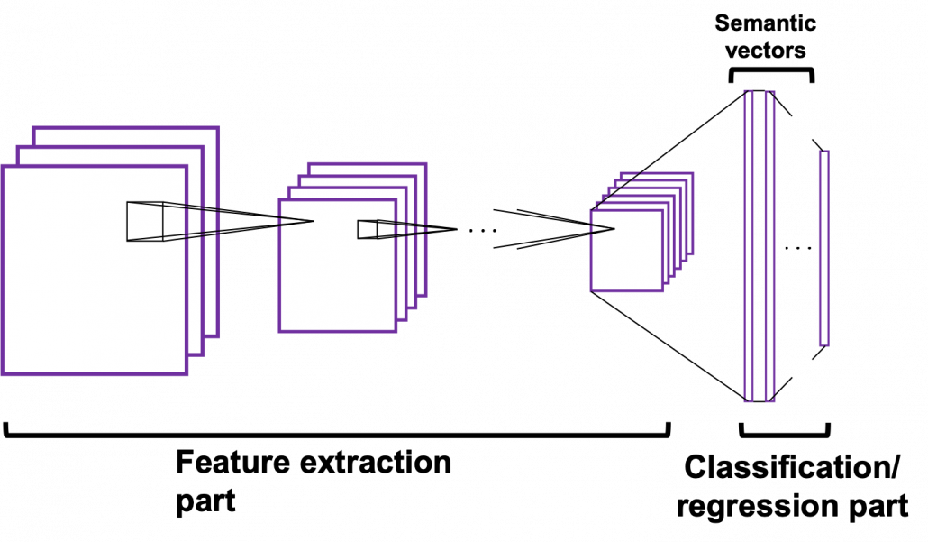
  are parameters. In case of classical machine learning algorithms, the number of those parameters are very limited because they were originally designed manually. Such functions for classical machine learning is useful for features found by humans, after trial and errors(feature engineering is a field of finding such effective features, manually). You adjust those parameters based on how different the outputs(estimated outcome of classification/regression) are from supervising vectors(the data prepared to show ideal answers).
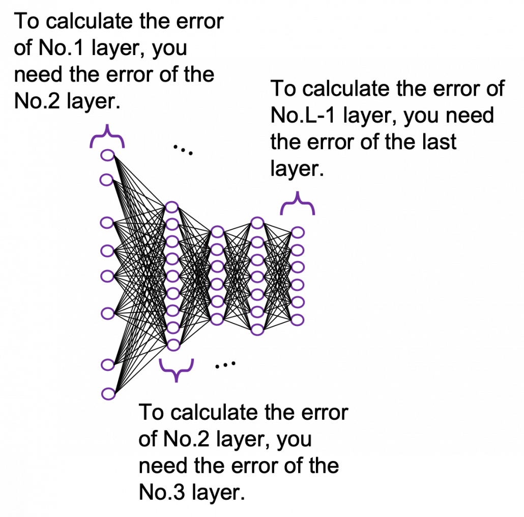
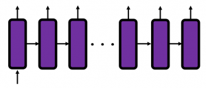
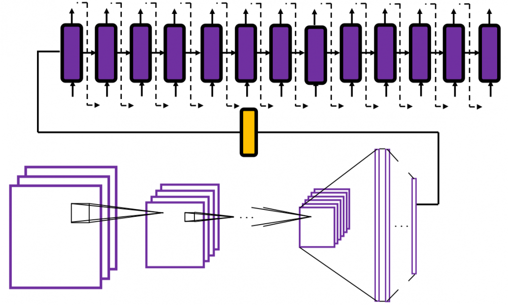
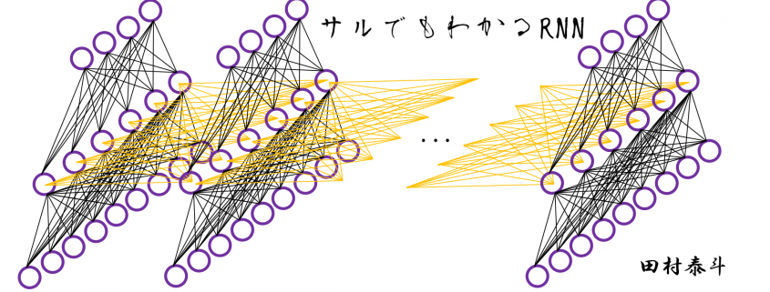
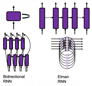
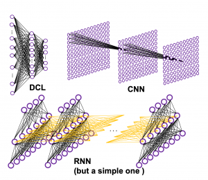
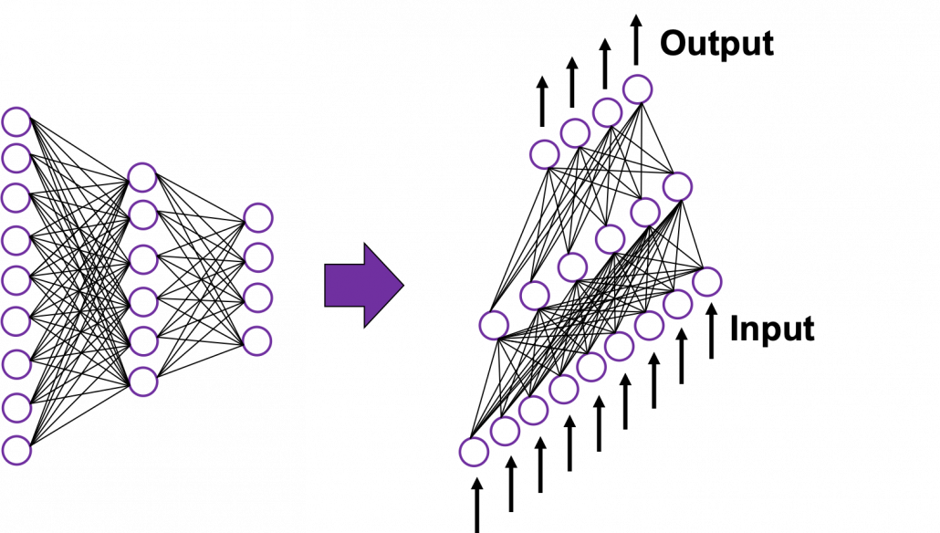 In fact the simple RNN which we are going to look at in this article has only three layers. From now on imagine that inputs of RNN come from the bottom and outputs go up. But RNNs have to keep information of earlier times steps during upcoming several time steps because as I mentioned in the last article RNNs are used for sequence data, the order of whose elements is important. In order to do that, information of the neurons in the middle layer of RNN propagate forward to the middle layer itself. Therefore in one time step of forward propagation of RNN, the input at the time step propagates forward as normal DCL, and the RNN gives out an output at the time step. And information of one neuron in the middle layer propagate forward to the other neurons like yellow arrows in the figure. And the information in the next neuron propagate forward to the other neurons, and this process is repeated. This is called recurrent connections of RNN.
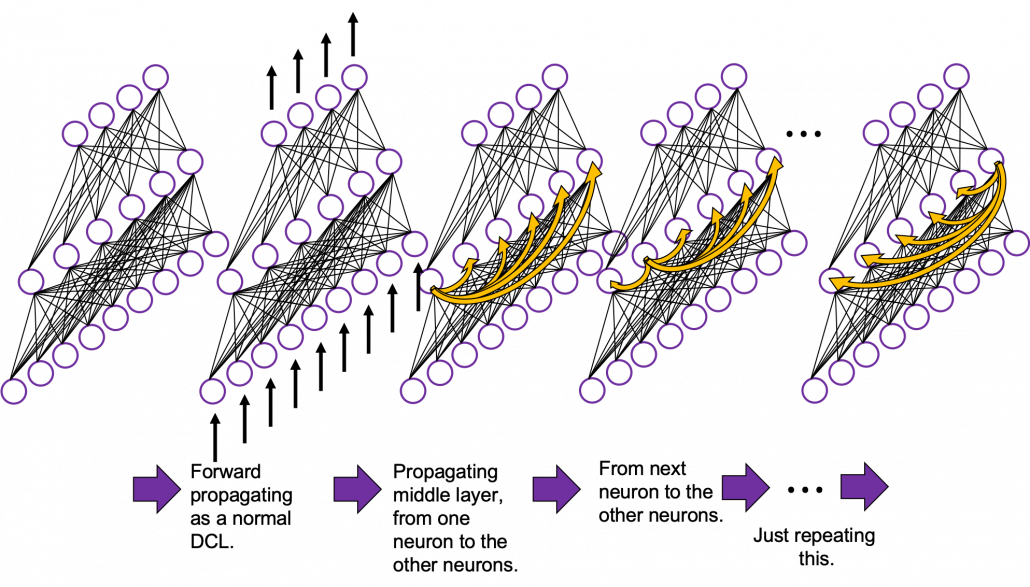
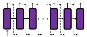
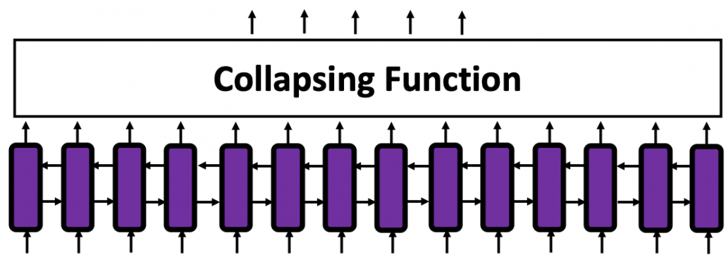
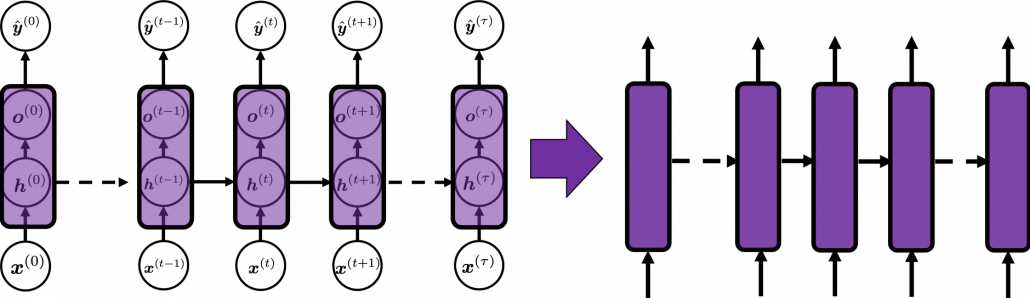
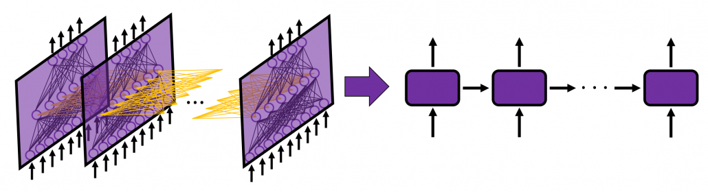
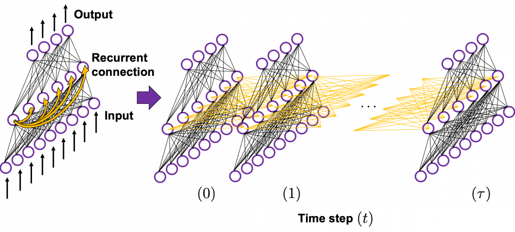 In many situations, RNNs are simplified as below. If you have read through this article until this point, I bet you gained some better understanding of RNNs, so you should little by little get used to this more abstract, blackboxed way of showing RNN.
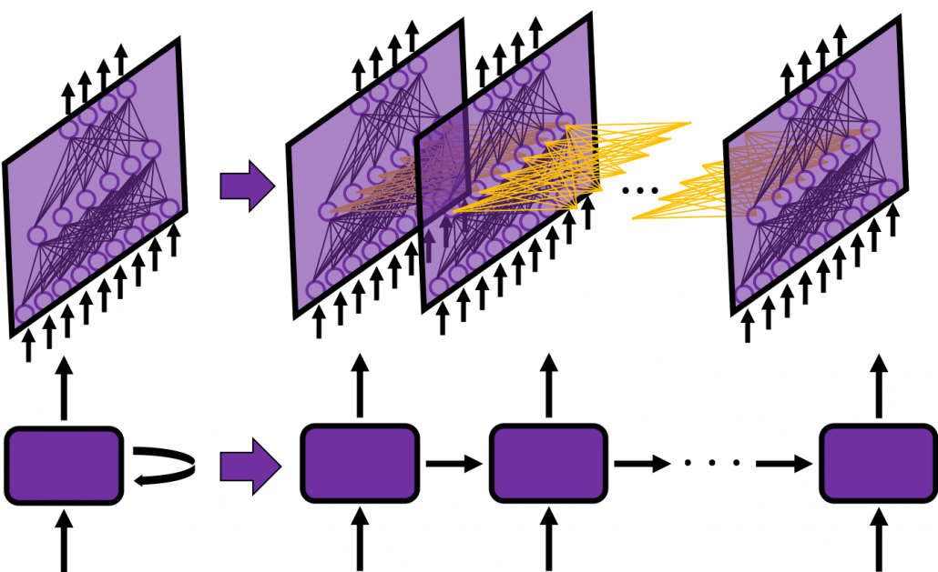
 .
.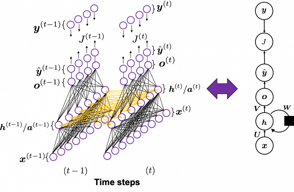
 at time step
 propagate forward as a normal DCL, and gives out the output
  (The notation on the
  is called “hat,” and it means that the value is an estimated value. Whatever machine learning tasks you work on, the outputs of the functions are just estimations of ideal outcomes. You need to adjust parameters for better estimations. You should always be careful whether it is an actual value or an estimated value in the context of machine learning or statistics). But the most important parts are the middle layers.
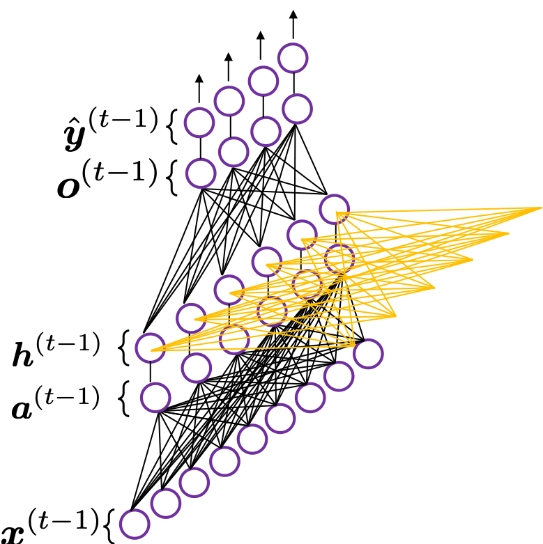
 is just linear summations of
  (If you do not know what “linear summations” mean, please scroll this page a bit), and
  is a combination of activated values of
  from the last time step, with recurrent connections. The values of
  , and the other is recurrent connections to
  .
.


 , and weights
  , then
  is a linear summation of
  , and its weights are
  .
. and
and  , you should clearly make an image of connections between two layers of a neural network. You can also say each element of
  is a linear summations all the elements of
  , and
, and 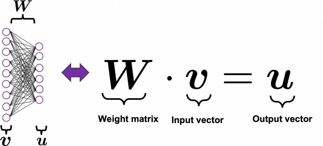
 , at every time step.
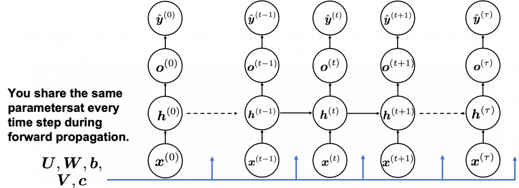
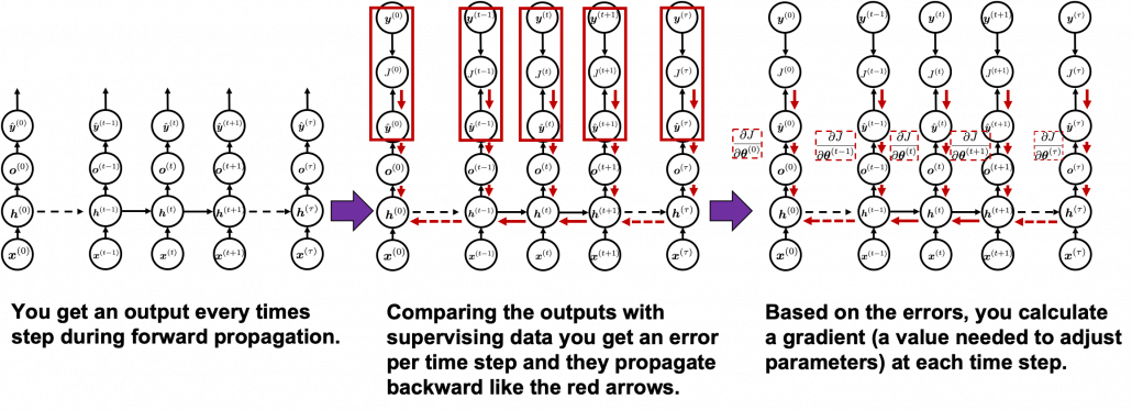 You need all the gradients to adjust parameters, but you do not necessarily need all the errors to calculate those gradients. Gradients in the context of machine learning mean partial derivatives of error functions (in this case
  ) with respect to certain parameters, and mathematically a gradient of
  is denoted as
  . And another confusing point in many textbooks, including the MIT one, is that they give an impression that parameters depend on time steps. For example some study materials use notations like
  , and I think this gives an impression that this is a gradient with respect to the parameters at time step
  . In my opinion this gradient rather should be written as
  . But many study materials denote gradients of those errors in the former way, so from now on let me use the notations which you can see in the figures in this article.
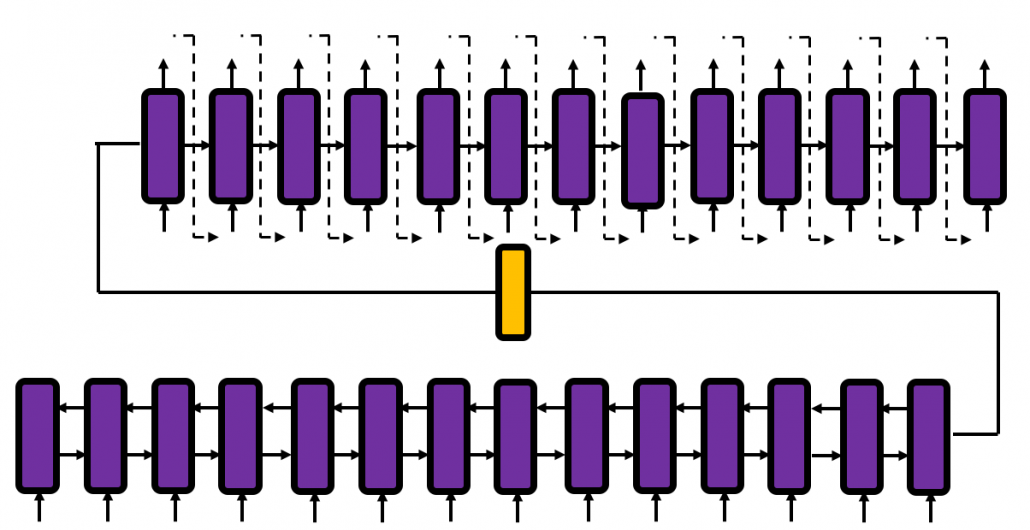
 you need errors from time steps
  (as you can see in the figure, in order to calculate a gradient in a colored frame, you need all the errors in the same color).
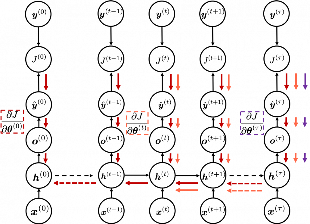
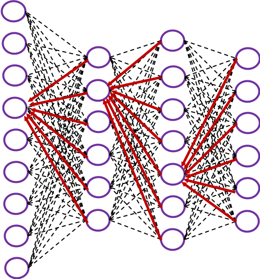
 different colors to show the whole process of RNN backprop, but that is not realistic. In the figure I displayed only the flows of errors necessary for calculating each gradient at time step
  .
. are correct notations, because
  are values of neurons after forward propagation. They depend on time steps, and these are very values which I have been calling “errors.” That is why parameters do not depend on time steps, whereas errors depend on time steps.
 . With this gradient
  , you can finally renew the value of
  one time.


 , which most people would have seen in compulsory education, is a part of mapping. If you get a value x, you get a value y corresponding to the x.
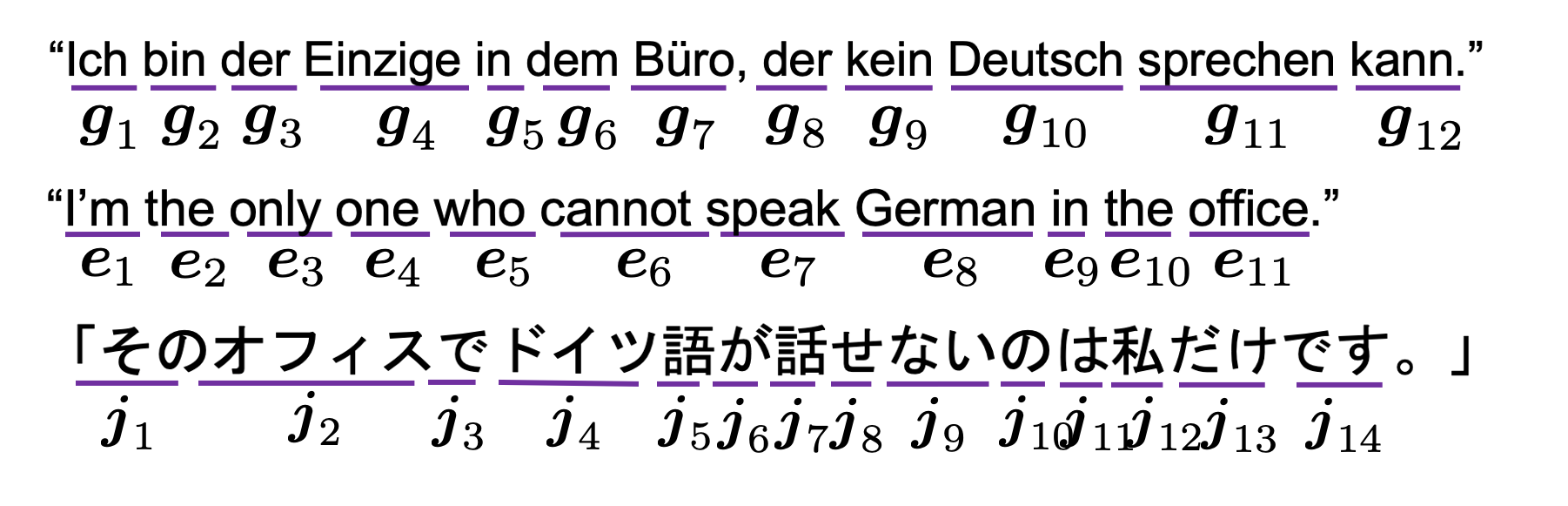

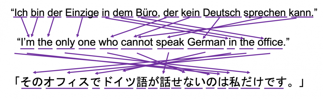
 , and machine translation is nothing but mappings between these sequence data.