Einführung und Vertiefung in R Statistics mit den Dortmunder R-Kursen!

May 19, 2020/0 Comments/in Carrier, Certification / Training, Education / Certification, Gerneral, R Statistics /by events

Im Rahmen der Dortmunder R Kurse bieten wir unsere Expertise in Schulungen für die Programmiersprache R an. Zielgruppe unserer Fortbildungen sind nicht nur Statistiker, sondern auch Anwender jeder Fachrichtung aus Industrie und Forschungseinrichtungen, die mit R ihre Daten analysieren wollen. Die Dortmunder R-Kurse werden ausschließlich von Statistikern mit langjähriger Erfahrung angeboten. Die Referenten gehören zum engsten Kreis der internationalen R-Gemeinschaft. Die angebotenen Kurse haben sich vielfach national und international bewährt.

Unsere Termine für die Online-Durchführung in diesem Jahr:

8., 9. und 10. Juni: R-Basiskurs (jeweils 9:00 – 14:00 Uhr)

22., 23., 24. und 25. Juni: R-Vertiefungskurs (jeweils 9:00 – 13:00 Uhr)

Kosten jeweils 750.00€, bei Buchung beider Kurse im Juni erhalten Sie einen Preisnachlass von 200€.

Zur Anmeldung gelangen Sie über den nachfolgenden Link:
https://www.zhb.tu-dortmund.de/zhb/wb/de/home/Seminare/Andere_Veranst/index.html

R Basiskurs

Das Seminar R Basiskurs für Anfänger findet am 8., 9. und 10. Juni 2020 statt. Den Teilnehmern wird der praxisrelevante Part der Programmiersprache näher gebracht, um so die Grundlagen zur ersten Datenanalyse — von Datensatz zu statistischen Kennzahlen und ersten Visualisierungen — zu schaffen. Anmeldeschluss ist der 25. Mai 2020.

Programm:

Installation von R und zugehöriger Entwicklungsumgebung
Grundlagen von R: Syntax, Datentypen, Operatoren, Funktionen, Indizierung
R-Hilfe effektiv nutzen
Ein- und Ausgabe von Daten
Behandlung fehlender Werte
Statistische Kennzahlen
Visualisierung

R Vertiefungskurs

Das Seminar R-Vertiefungskurs für Fortgeschrittene findet am 22., 23., 24. und 25. Juni (jeweils von 9:00 – 13:00 Uhr) statt. Die Veranstaltung ist ideal für Teilnehmende mit ersten Vorkenntnissen, die ihre Analysen effizient mit R durchführen möchten. Anmeldeschluss ist der 11. Juni 2020.

Der Vertiefungskurs baut inhaltlich auf dem Basiskurs auf. Es besteht aber keine Verpflichtung, bei Besuch des Vertiefungskurses zuvor den Basiskurs zu absolvieren, wenn bereits entsprechende Vorkenntnisse in R vorhanden sind.

Programm:

Eigene Funktionen, Schleifen vermeiden durch *apply
Einführung in ggplot2 und dplyr
Statistische Tests und Lineare Regression
Dynamische Berichterstellung
Angewandte Datenanalyse anhand von Fallbeispielen

Links zur Veranstaltung direkt:

R-Basiskurs: https://dortmunder-r-kurse.de/kurse/r-basiskurs/

R-Vertiefungskurs: https://dortmunder-r-kurse.de/kurse/r-vertiefungskurs/

Python vs R: Which Language to Choose for Deep Learning?

February 18, 2020/1 Comment/in Data Mining, Data Science, Insights, Python, R Statistics /by Deep Moteria

Data science is increasingly becoming essential for every business to operate efficiently in this modern world. This influences the processes composed together to obtain the required outputs for clients. While machine learning and deep learning sit at the core of data science, the concepts of deep learning become essential to understand as it can help increase the accuracy of final outputs. And when it comes to data science, R and Python are the most popular programming languages used to instruct the machines.

Python and R: Primary Languages Used for Deep Learning

Deep learning and machine learning differentiate based on the input data type they use. While machine learning depends upon the structured data, deep learning uses neural networks to store and process the data during the learning. Deep learning can be described as the subset of machine learning, where the data to be processed is defined in another structure than a normal one.

R is developed specifically to support the concepts and implementation of data science and hence, the support provided by this language is incredible as writing codes become much easier with its simple syntax.

Python is already much popular programming language that can serve more than one development niche without straining even for a bit. The implementation of Python for programming machine learning algorithms is very much popular and the results provided are accurate and faster than any other language. (C or Java). And because of its extended support for data science concept implementation, it becomes a tough competitor for R.

However, if we compare the charts of popularity, Python is obviously more popular among data scientists and developers because of its versatility and easier usage during algorithm implementation. However, R outruns Python when it comes to the packages offered to developers specifically expertise in R over Python. Therefore, to conclude which one of them is the best, let’s take an overview of the features and limits offered by both languages.

Python

Python was first introduced by Guido Van Rossum who developed it as the successor of ABC programming language. Python puts white space at the center while increasing the readability of the developed code. It is a general-purpose programming language that simply extends support for various development needs.

The packages of Python includes support for web development, software development, GUI (Graphical User Interface) development and machine learning also. Using these packages and putting the best development skills forward, excellent solutions can be developed. According to Stackoverflow, Python ranks at the fourth position as the most popular programming language among developers.

Benefits for performing enhanced deep learning using Python are:

Concise and Readable Code
Extended Support from Large Community of Developers
Open-source Programming Language
Encourages Collaborative Coding
Suitable for small and large-scale products

The latest and stable version of Python has been released as Python 3.8.0 on 14th October 2019. Developing a software solution using Python becomes much easier as the extended support offered through the packages drives better development and answers every need.

R

R is a language specifically used for the development of statistical software and for statistical data analysis. The primary user base of R contains statisticians and data scientists who are analyzing data. Supported by R Foundation for statistical computing, this language is not suitable for the development of websites or applications. R is also an open-source environment that can be used for mining excessive and large amounts of data.

R programming language focuses on the output generation but not the speed. The execution speed of programs written in R is comparatively lesser as producing required outputs is the aim not the speed of the process. To use R in any development or mining tasks, it is required to install its operating system specific binary version before coding to run the program directly into the command line.

R also has its own development environment designed and named RStudio. R also involves several libraries that help in crafting efficient programs to execute mining tasks on the provided data.

The benefits offered by R are pretty common and similar to what Python has to offer:

Open-source programming language
Supports all operating systems
Supports extensions
R can be integrated with many of the languages
Extended Support for Visual Data Mining

Although R ranks at the 17th position in Stackoverflow’s most popular programming language list, the support offered by this language has no match. After all, the R language is developed by statisticians for statisticians!

Python vs R: Should They be Really Compared?

Even when provided with the best technical support and efficient tools, a developer will not be able to provide quality outputs if he/she doesn’t possess the required skills. The point here is, technical skills rank higher than the resources provided. A comparison of these two programming languages is not advisable as they both hold their own set of advantages. However, the developers considering to use both together are less but they obtain maximum benefit from the process.

Both these languages have some features in common. For example, if a representative comes asking you if you lend technical support for developing an uber clone, you are directly going to decline as Python and R both do not support mobile app development. To benefit the most and develop excellent solutions using both these programming languages, it is advisable to stop comparing and start collaborating!

R and Python: How to Fit Both In a Single Program

Anticipating the future needs of the development industry, there has been a significant development to combine these both excellent programming languages into one. Now, there are two approaches to performing this: either we include R script into Python code or vice versa.

Using the available interfaces, packages and extended support from Python we can include R script into the code and enhance the productivity of Python code. Availability of PypeR, pyRserve and more resources helps run these two programming languages efficiently while efficiently performing the background work.

Either way, using the developed functions and packages made available for integrating Python in R are also effective at providing better results. Available R packages like rJython, rPython, reticulate, PythonInR and more, integrating Python into R language is very easy.

Therefore, using the development skills at their best and maximizing the use of such amazing resources, Python and R can be togetherly used to enhance end results and provide accurate deep learning support.

Conclusion

Python and R both are great in their own names and own places. However, because of the wide applications of Python in almost every operation, the annual packages offered to Python developers are less than the developers skilled in using R. However, this doesn’t justify the usability of R. The ultimate decision of choosing between these two languages depends upon the data scientists or developers and their mining requirements.

And if a developer or data scientist decides to develop skills for both- Python and R-based development, it turns out to be beneficial in the near future. Choosing any one or both to use in your project depends on the project requirements and expert support on hand.

Multi-touch attribution: A data-driven approach

February 4, 2020/1 Comment/in Data Science, Gerneral, Insights, Python, R Statistics, Tutorial, Use Case, Use Cases, Visualization /by Aakash Chugh

This is the first article of article series Getting started with the top eCommerce use cases.

What is Multi-touch attribution?

Customers shopping behavior has changed drastically when it comes to online shopping, as nowadays, customer likes to do a thorough market research about a product before making a purchase. This makes it really hard for marketers to correctly determine the contribution for each marketing channel to which a customer was exposed to. The path a customer takes from his first search to the purchase is known as a Customer Journey and this path consists of multiple marketing channels or touchpoints. Therefore, it is highly important to distribute the budget between these channels to maximize return. This problem is known as multi-touch attribution problem and the right attribution model helps to steer the marketing budget efficiently. Multi-touch attribution problem is well known among marketers. You might be thinking that if this is a well known problem then there must be an algorithm out there to deal with this. Well, there are some traditional models but every model has its own limitation which will be discussed in the next section.

Traditional attribution models

Most of the eCommerce companies have a performance marketing department to make sure that the marketing budget is spent in an agile way. There are multiple heuristics attribution models pre-existing in google analytics however there are several issues with each one of them. These models are:

First touch attribution model

100% credit is given to the first channel as it is considered that the first marketing channel was responsible for the purchase.

Figure 1: First touch attribution model

Last touch attribution model

100% credit is given to the last channel as it is considered that the first marketing channel was responsible for the purchase.

Figure 2: Last touch attribution model

Linear-touch attribution model

In this attribution model, equal credit is given to all the marketing channels present in customer journey as it is considered that each channel is equally responsible for the purchase.

Figure 3: Linear attribution model

U-shaped or Bath tub attribution model

This is most common in eCommerce companies, this model assigns 40% to first and last touch and 20% is equally distributed among the rest.

Figure 4: Bathtub or U-shape attribution model

Data driven attribution models

Traditional attribution models follows somewhat a naive approach to assign credit to one or all the marketing channels involved. As it is not so easy for all the companies to take one of these models and implement it. There are a lot of challenges that comes with multi-touch attribution problem like customer journey duration, overestimation of branded channels, vouchers and cross-platform issue, etc.

Switching from traditional models to data-driven models gives us more flexibility and more insights as the major part here is defining some rules to prepare the data that fits your business. These rules can be defined by performing an ad hoc analysis of customer journeys. In the next section, I will discuss about Markov chain concept as an attribution model.

Markov chains

Markov chains concepts revolves around probability. For attribution problem, every customer journey can be seen as a chain(set of marketing channels) which will compute a markov graph as illustrated in figure 5. Every channel here is represented as a vertex and the edges represent the probability of hopping from one channel to another. There will be an another detailed article, explaining the concept behind different data-driven attribution models and how to apply them.

Figure 5: Markov chain example

Challenges during the Implementation

Transitioning from a traditional attribution models to a data-driven one, may sound exciting but the implementation is rather challenging as there are several issues which can not be resolved just by changing the type of model. Before its implementation, the marketers should perform a customer journey analysis to gain some insights about their customers and try to find out/perform:

Length of customer journey.
On an average how many branded and non branded channels (distinct and non-distinct) in a typical customer journey?
Identify most upper funnel and lower funnel channels.
Voucher analysis: within branded and non-branded channels.

When you are done with the analysis and able to answer all of the above questions, the next step would be to define some rules in order to handle the user data according to your business needs. Some of the issues during the implementation are discussed below along with their solution.

Customer journey duration

Assuming that you are a retailer, let’s try to understand this issue with an example. In May 2016, your company started a Fb advertising campaign for a particular product category which “attracted” a lot of customers including Chris. He saw your Fb ad while working in the office and clicked on it, which took him to your website. As soon as he registered on your website, his boss called him (probably because he was on Fb while working), he closed everything and went for the meeting. After coming back, he started working and completely forgot about your ad or products. After a few days, he received an email with some offers of your products which also he ignored until he saw an ad again on TV in Jan 2019 (after 3 years). At this moment, he started doing his research about your products and finally bought one of your products from some Instagram campaign. It took Chris almost 3 years to make his first purchase.

Figure 6: Chris journey

Now, take a minute and think, if you analyse the entire journey of customers like Chris, you would realize that you are still assigning some of the credit to the touchpoints that happened 3 years ago. This can be solved by using an attribution window. Figure 6 illustrates that 83% of the customers are making a purchase within 30 days which means the attribution window here could be 30 days. In simple words, it is safe to remove the touchpoints that happens after 30 days of purchase. This parameter can also be changed to 45 days or 60 days, depending on the use case.

Figure 7: Length of customer journey

Removal of direct marketing channel

A well known issue that every marketing analyst is aware of is, customers who are already aware of the brand usually comes to the website directly. This leads to overestimation of direct channel and branded channels start getting more credit. In this case, you can set a threshold (say 7 days) and remove these branded channels from customer journey.

Figure 8: Removal of branded channels

Cross platform problem

If some of your customers are using different devices to explore your products and you are not able to track them then it will make retargeting really difficult. In a perfect world these customers belong to same journey and if these can’t be combined then, except one, other paths would be considered as “non-converting path”. For attribution problem device could be thought of as a touchpoint to include in the path but to be able to track these customers across all devices would still be challenging. A brief introduction to deterministic and probabilistic ways of cross device tracking can be found here.

Figure 9: Cross platform clash

How to account for Vouchers?

To better account for vouchers, it can be added as a ‘dummy’ touchpoint of the type of voucher (CRM,Social media, Affiliate or Pricing etc.) used. In our case, we tried to add these vouchers as first touchpoint and also as a last touchpoint but no significant difference was found. Also, if the marketing channel of which the voucher was used was already in the path, the dummy touchpoint was not added.

Figure 10: Addition of Voucher as a touchpoint

Let me know in comments if you would like to add something or if you have a different perspective about this use case.

Getting started with the top eCommerce use cases

January 13, 2020/0 Comments/in Business Analytics, Data Science, Machine Learning, Python, R Statistics, Use Case /by Aakash Chugh

Nowadays, almost all the projects in eCommerce companies are data-dependent and everyone wants to leverage data science techniques to mine as much information as they can from that data. From tracking their customer’s shopping behavior to recommending them what to buy, from finding new leads for their market to calculating their lifetime value, from improving customer experience to increase their profitability. When we navigate through any website, we leave our traces and companies track these touchpoints to get insights about how we behave online. Companies sometimes have different landing pages based on the gender of the user.

This post will be focused on some of the use cases in marketing which are gaining attention over the past few years. I have been associated with different eCommerce companies as a data science consultant.

Upcoming months has a lot to offer as I will be writing blogs about the following use cases:

Multi-touch attribution: A data-driven approach
Introduction to Recommendation engines
How Important is Customer Lifetime Value?
Customer Segmentation
Dynamic Pricing

If you are interested in reading the success story for the Multi-touch attribution project you can find it here.

A common trap when it comes to sampling from a population that intrinsically includes outliers

February 21, 2019/0 Comments/in Business Analytics, Business Intelligence, Data Mining, Data Science, Data Science Hack, Main Category, R Statistics, Statistics /by Moussa El-Zaarah

I will discuss a common fallacy concerning the conclusions drawn from calculating a sample mean and a sample standard deviation and more importantly how to avoid it.

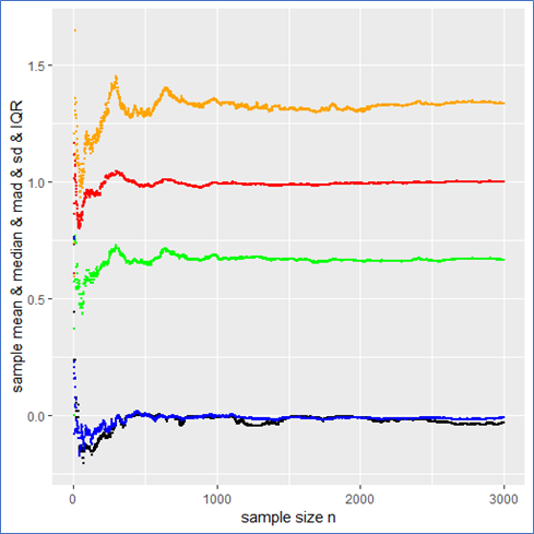
Suppose you draw a random sample $x_1$ , $x_2$ , … $x_N$ of size $N$ and compute the ordinary (arithmetic) sample mean $x_m$ and a sample standard deviation $sd$ from it. Now if (and only if) the (true) population mean µ (first moment) and population variance (second moment) obtained from the actual underlying PDF are finite, the numbers $x_m$ and $sd$ make the usual sense otherwise they are misleading as will be shown by an example.

By the way: The common correlation coefficient will also be undefined (or in practice always point to zero) in the presence of infinite population variances. Hopefully I will create an article discussing this related fallacy in the near future where a suitable generalization to Lévy-stable variables will be proposed.

Drawing a random sample from a heavy tailed distribution and discussing certain measures

As an example suppose you have a one dimensional random walker whose step length is distributed by a symmetric standard Cauchy distribution (Lorentz-profile) with heavy tails, i.e. an alpha-stable distribution with alpha being equal to one. The PDF of an individual independent step is given by $p(x) = \frac{\pi^{-1}}{(1 + x^2)}$ , thus neither the first nor the second moment exist whereby the first exists and vanishes at least in the sense of a principal value due to symmetry.

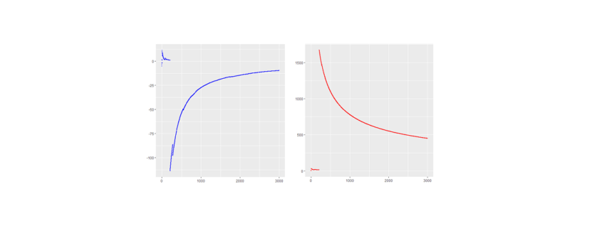
Still let us generate $N = 3000$ (pseudo) standard Cauchy random numbers in R* to analyze the behavior of their sample mean and standard deviation $sd$ as a function of the reduced sample size $n \leq N$ .

*The R-code is shown at the end of the article.

Here are the piecewise sample mean (in blue) and standard deviation (in red) for the mentioned Cauchy sampling. We see that both the sample mean and $sd$ include jumps and do not converge.

Especially the mean deviates relatively largely from zero even after 3000 observations. The sample $sd$ has no target due to the population variance being infinite.

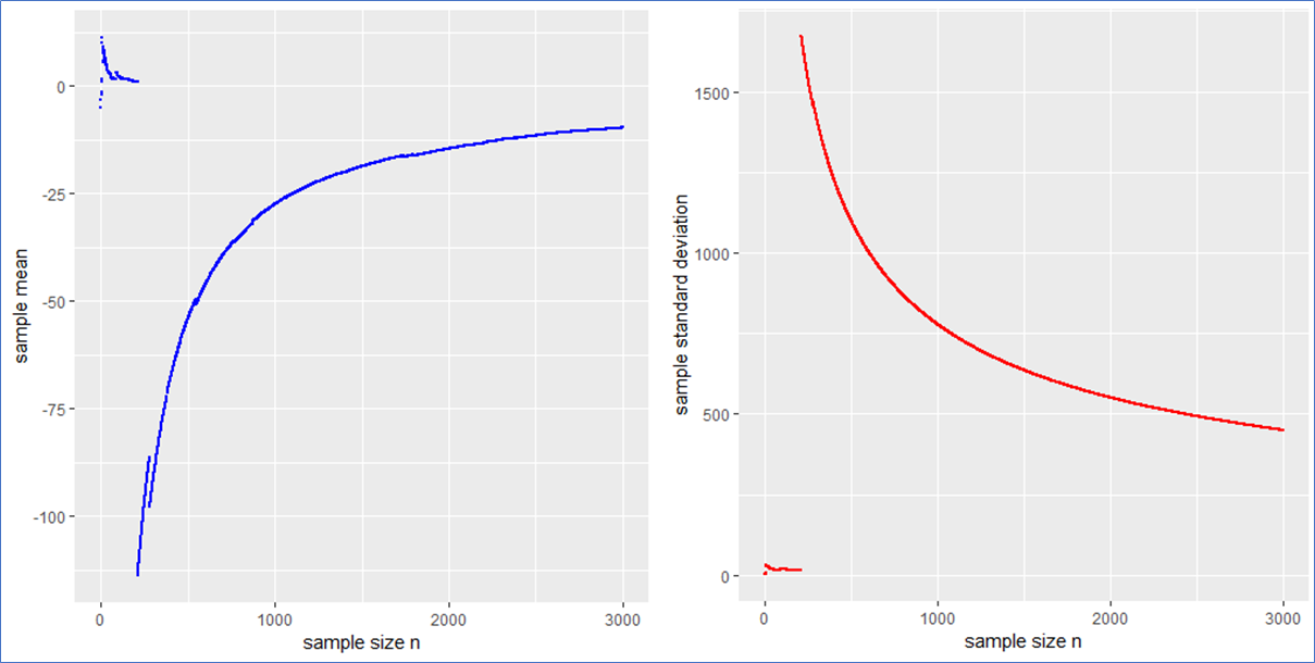
If the data is new and no prior distribution is known, computing the sample mean and $sd$ will be misleading. Astonishingly enough the sample mean itself will have the (formally exact) same distribution as the single step length $p(x)$ . This means that the sample mean is also standard Cauchy distributed implying that with a different Cauchy sample one could have easily observed different sample means far of the presented values in blue.

What sense does it make to present the usual interval $x_m \pm sd / \sqrt{N}$ in such a case? What to do?

The sample median, median absolute difference (mad) and Inter-Quantile-Range (IQR) are more appropriate to describe such a data set including outliers intrinsically. To make this plausible I present the following plot, whereby the median is shown in black, the mad in green and the IQR in orange.

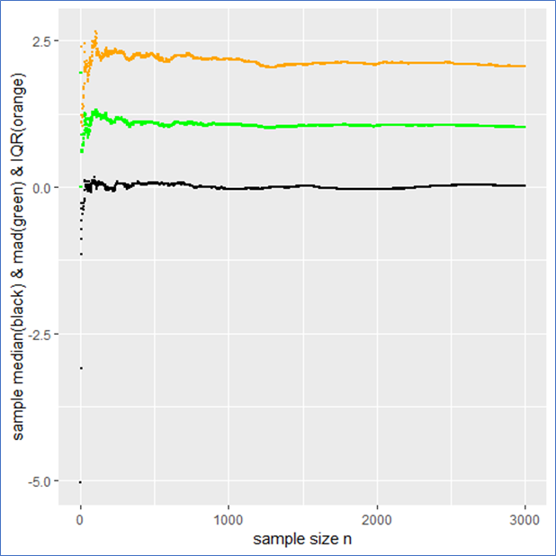
This example shows that the median, mad and IQR converge quickly against their assumed values and contain no major jumps. These quantities do an obviously better job in describing the sample. Even in the presence of outliers they remain robust, whereby the mad converges more quickly than the IQR. Note that a standard Cauchy sample will contain half of its sample in the interval median $\pm$ mad meaning that the IQR is twice the mad.

Drawing a random sample from a PDF that has finite moments

Just for comparison I also show the above quantities for a standard normal (pseudo) sample labeled with the same color as before as a counter example. In this case not only do both the sample mean and median but also the $sd$ and mad converge towards their expected values (see plot below). Here all the quantities describe the data set properly and there is no trap since there are no intrinsic outliers. The sample mean itself follows a standard normal, so that the $sd$ in deed makes sense and one could calculate a standard error $\frac{sd}{\sqrt{N}}$ from it to present the usual stochastic confidence intervals for the sample mean.

A careful observation shows that in contrast to the Cauchy case here the sampled mean and $sd$ converge more quickly than the sample median and the IQR. However still the sampled mad performs about as well as the $sd$ . Again the mad is twice the IQR.

And here are the graphs of the prementioned quantities for a pseudo normal sample:

The take-home-message:

Just be careful when you observe outliers and calculate sample quantities right away, you might miss something. At best one carefully observes how the relevant quantities change with sample size as demonstrated in this article.

Such curves should become of broader interest in order to improve transparency in the Data Science process and reduce fallacies as well.

Thank you for reading.

P.S.: Feel free to play with the set random seed in the R-code below and observe how other quantities behave with rising sample size. Of course you can also try different PDFs at the beginning of the code. You can employ a Cauchy, Gaussian, uniform, exponential or Holtsmark (pseudo) random sample.

QUIZ: Which one of the recently mentioned random samples contains a trap** and why?

**in the context of this article

R-code used to generate the data and for producing plots:

1

2

3

4

5

6

7

8

9

10

11

12

13

14

15

16

17

18

19

20

21

22

23

24

25

26

27

28

29

30

31

32

33

34

35

36

37

38

39

40

41

42

43

44

45

46

47

48

49

50

51

52

53

54

55

56

57

58

59

60

61

62

63

64

65

66

67

68

69

70

71

72

73

74

75

76

77

78

79

80

81

82

83

84

85

86

87

88

89

90

91

92

93

94

95

96

97

#R-script for emphasizing convergence and divergence of sample means

####install and load relevant packages ####

#uncomment these lines if necessary

#install.packages(c('ggplot2',’stabledist’))

#library(ggplot2)

#library(stabledist)

#####drawing random samples #####

#Setting a random seed for being able to reproduce results

set.seed(1234567)

N= 2000 #sample size

#Choose a PDF from which a sample shall be drawn

#To do so (un)comment the respective lines of following code

data <- rcauchy(N) # option1(default): standard Cauchy sampling

#data <- rnorm(N) #option2: standard Gaussian sampling

#data <- rexp(N) # option3: standard exponential sampling

#data <- rstable(N,alpha=1.5,beta=0) # option4: standard symmetric Holtsmark sampling

#data <- runif(N) #option5: standard uniform sample

#####descriptive statistics####

#preparations/declarations

SUM = vector()

sd =vector()

mean = vector()

SQ =vector()

SQUARES = vector()

median = vector()

mad =vector()

quantiles = data.frame()

sem =vector()

#piecewise calculaion of descrptive quantities

for (k in 1:length(data)){ #mainloop

SUM[k] <- sum(data[1:k]) # sum of sample

mean[k] <- mean(data[1:k]) # arithmetic mean

sd[k] <- sd(data[1:k]) # standard deviation

sem[k] <- sd[k]/(sqrt(k)) #standard error of the sample mean (for finite variances)

mad[k] <- mad(data[1:k],const=1) # median absolute deviation

for (j in 1:5){

qq <- quantile(data[1:k],na.rm = T)

quantiles[k,j] <- qq[j] #quantiles of sample

}

colnames(quantiles) <- c('min','Q1','median','Q3','max')

for (i in 1:length(data[1:k])){

SQUARES[i] <- data[i]*data[i]

}

SQ[k] <- sum(SQUARES[1:k]) #sum of squares of random sample

} #end of mainloop

#create table containing all relevant data

TABLE <- as.data.frame(cbind(quantiles,mean,sd,SQ,SUM,sem))

#####plotting results###

x11()

print(ggplot(TABLE,aes(1:N,median))+

geom_point(size=.5)+xlab('sample size n')+ylab('sample median'))

x11()

print(ggplot(TABLE,aes(1:N,mad))+geom_point(size=.5,color ='green')+

xlab('sample size n')+ylab('sample median absolute difference'))

x11()

print(ggplot(TABLE,aes(1:N,sd))+geom_point(size=.5,color ='red')+

xlab('sample size n')+ylab('sample standard deviation'))

x11()

print(ggplot(TABLE,aes(1:N,mean))+geom_point(size=.5, color ='blue')+

xlab('sample size n')+ylab('sample mean'))

x11()

print(ggplot(TABLE,aes(1:N,Q3-Q1))+geom_point(size=.5, color ='blue')+

xlab('sample size n')+ylab('IQR'))

#uncomment the following lines of code to see further plots

#x11()

#print(ggplot(TABLE,aes(1:N,sem))+geom_point(size=.5)+

#xlab('sample size n')+ylab('sample sum of r.v.'))

#x11()

#print(ggplot(TABLE,aes(1:N,SUM))+geom_point(size=.5)+

#xlab('sample size n')+ylab('sample sum of r.v.'))

#x11()

#print(ggplot(TABLE,aes(1:N,SQ))+geom_point(size=.5)+

#xlab('sample size n')+ylab('sample sum of squares'))

Cross-industry standard process for data mining

January 17, 2019/0 Comments/in Data Engineering, Data Mining, Data Science, Data Science Hack, Data Science News, Machine Learning, Python, R Statistics /by Aakash Chugh

Introduced in 1996, the cross-industry standard process for data mining (CRISP-DM) became the most
common procedure for all data mining projects. This method consists of six phases: Business
understanding, Data understanding, Data preparation, Modeling, Evaluation and Deployment (see
Figure 1). It is being used not just as a reference manual but as a user guide as it explains every phase
in detail (Hipp, 2000). The six phases of this model are explained below:

Figure 1: Different phases of CRISP-DM

Business Understanding

It includes understanding the business problem and determining the
objective of the business as well as of the project. It is also important to understand the previous work
done on the project (if any) to achieve the business goals and to examine if the scope of the project has changed.

The job of a Data Scientist is not limited to coding or just make a machine learning model and I guess that’s why this whole lifecycle was developed. The key points a project owner should take care in this process are:

– Identify stakeholders and involve them to define the scope your project
– Describe your product (your machine learning model)
– Identify how your product ties into the client’s business processes
– Identify metrics / KPIs for measuring success

Evaluating a model is a different thing as it can only tell you how good are your predictions but identifying the success metric is really important for any data science project because when your model is deployed in production this measure will tell you if your model actually works or not. Now, let’s discuss what is this success metric

Consider that you are working in an e-commerce company where Head of finance ask you to create a machine learning model to predict if a specific product will return or not. The problem is not hard to understand, its a binary classification problem and you know you can do the job. But before you start working with the data you should define a metric to measure the success. What do you think your success metric could be? I would go with the return rate, in other words, calculate the rate for how many orders are actually coming back and if this measure is getting decrease you would know your model works and if not then FIX IT !!

Data understanding

The initial step in this phase is to gather all the data from different sources. It is
then important to describe the data, generate graphs for distribution in order to get familiar with the
data. This phase is important as without enough data or without understanding about the data analysis
cannot be performed. In data mining terms this can be compared to Exploratory data analysis (EDA)
where techniques from descriptive statistics are used to have an insight into the data. For instance, if it is
a time series data it makes sense to know from when until when the data is available before diving deep into
the data.

Data preparation

This phase takes most of the time in data mining project as a lot of methods from
data cleaning, feature subset, feature engineering, the transformation of data etc. are used before the final
dataset is trained for modeling purpose. The single dataset can also be prepared in different forms as some
algorithms can learn more with a certain type of data, some algorithms can deal with imbalance dataset
and for some algorithms, the target variable must be balanced. This phase also requires sometimes to
calculate new KPI’s according to the business need or sometimes to reduce the dimension of the dataset.

Modeling and Evaluation

Various models are selected and build in this process and appropriate hyperparameters are
selected after an intensive grid search. Once all the models are built it is now time to evaluate and compare performances of all the models.

Deployment

A model is of no use if it is not deployed into production. Until now you have been doing the job of a data scientist but for deployment, you need some software engineering

skills. There are several ways to deploy a machine learning model or python code. Few of them are:

Re-implement your python code in C++, Java etc. (LOL)
Save the coefficients and use them to get predictions
Serialized objects (REST API with flask, Django)

To understand the concept of deploying an ML model using REST API this post is highly recommended.

Fuzzy Matching mit dem Jaro-Winkler-Score zur Auswertung von Markenbekanntheit und Werbeerinnerung

December 10, 2018/0 Comments/in Business Analytics, Data Mining, Data Science, Data Science Hack, Main Category, R Statistics, Text Mining /by Markus Lang

Für Unternehmen sind Markenbekanntheit und Werbeerinnerung wichtige Zielgrößen, denn anhand dieser lässt sich ableiten, ob Konsumenten ein Produkt einer Marke kaufen werden oder nicht. Zielgrößen wie diese werden von Marktforschungsinstituten über Befragungen ermittelt. Dafür wird in regelmäßigen Zeitabständen eine gleichbleibende Anzahl an Personen befragt, ob diese sich an Marken einer bestimmten Branche erinnern oder sich an Werbung erinnern. Die Personen füllen dafür in der Regel einen Onlinefragebogen aus.

Die Ergebnisse der Befragung liegen in einer Datenmatrix (siehe Tabelle) vor und müssen zur Auswertung zunächst bearbeitet werden.

Laufende Nummer	Marke 1	Marke 2	Marke 3	Marke 4
1	ING-Diba	Citigroup	Sparkasse
2	Sparkasse	Consorsbank
3	Commerbank	Deutsche Bank	Sparkasse	ING-DiBa
4	Sparkasse	Targobank

Ziel ist es aus diesen Daten folgende 0/1 codierte Matrix zu generieren. Wenn eine Marke bekannt ist, wird in die zur Marke gehörende Spalte eine Eins eingetragen, ansonsten eine Null.

Alle Marken	ING-Diba	Citigroup	Sparkasse	Targobank
ING-Diba, Citigroup, Sparkasse	1	1	1	0
Sparkasse, Consorsbank	0	0	1	0
Commerzbank, Deutsche Bank, Sparkasse, ING-Diba	1	0	0	0
Sparkasse, Targobank	0	0	1	1

Der Workflow um diese Datentransformation durchzuführen ist oftmals mittels eines Teilstrings einer Marke zu suchen ob diese in einem über alle Nennungen hinweg zusammengeführten String vorkommt oder nicht (z.B. „argo“ bei Targobank). Das Problem dieser Herangehensweise ist, dass viele falsch geschriebenen Wörter so nicht erfasst werden und die Erfahrung zeigt, dass falsch geschriebene Marken in vielfältigster Weise auftreten. Hier mussten in der Vergangenheit Mitarbeiter sich in stundenlangem Kampf durch die Ergebnisse wühlen und falsch zugeordnete oder nicht zugeordnete Marken händisch korrigieren und alle Variationen der Wörter notieren, um für die nächste Befragung das Suchpattern zu optimieren.

Eine Alternative diesen aufwändigen Workflow stellt die Ermittlung von falsch geschriebenen Wörtern mittels des Jaro-Winkler-Scores dar. Dafür muss zunächst die Jaro-Winkler-Distanz zwischen zwei Strings berechnet werden. Diese berechnet sich wie folgt:

$d_j = \frac{1}{3}(\frac{m}{|s_1|}+\frac{m}{|s_2|}+\frac{m - t}{m})$

m: Anzahl der übereinstimmenden Buchstaben
s: Länge des Strings
t: Hälfte der Anzahl der Umstellungen der Buchstaben die nötig sind, damit Strings identisch sind. („Ta“ und „gobank“ befinden sich bereits in der korrekten Reihenfolge, somit gilt: t = 0)

Aus dem Ergebnis lässt sich der Jaro-Winkler Score berechnen:
$d_w = \d_j + (l_p (1 - d_j))$
ist dabei die Jaro-Winkler-Distanz, l die Länge der übereinstimmenden Buchstaben von Beginn des Wortes bis zum maximal vierten Buchstaben und p ein konstanter Faktor von 0,1.

Für die Strings „Targobank“ und „Tangobank“ ergibt sich die Jaro-Winkler-Distanz:

$d_j = \frac{1}{3}(\frac{8}{9}+\frac{8}{9}+\frac{8 - 0}{9})$

Daraus wird im nächsten Schritt der Jaro-Winkler Score berechnet:

$d_w = 0,9259 + (2 \cdot 0,1 (1 - 0,9259)) = 0,9407407$

Bisherige Erfahrungen haben gezeigt, dass sich Scores ab 0,8 bzw. 0,9 am besten zur Suche von ähnlichen Wörtern eignen. Ein Schwellenwert darunter findet sehr viele Wörter, die sich z.B. auch anderen Wörtern zuordnen lassen. Ein Schwellenwert über 0,9 identifiziert falsch geschriebene Wörter oftmals nicht mehr.

Nach diesem theoretischen Exkurs möchte ich nun zeigen, wie sich das Ganze praktisch anwenden lässt. Da sich das Ganze um ein fiktives Beispiel handelt, werden zur Demonstration der Praxistauglichkeit Fakedaten mit folgendem Code erzeugt. Dabei wird angenommen, dass Personen unterschiedlich viele Banken kennen und diese mit einer bestimmten Wahrscheinlichkeit falsch schreiben.

1

2

3

4

5

6

7

8

9

10

11

12

13

14

15

16

17

18

19

20

21

22

23

24

25

26

27

28

29

30

31

32

33

34

35

36

37

38

39

40

41

42

43

44

45

46

47

48

49

50

51

52

53

54

55

56

57

58

59

60

61

62

63

64

65

66

67

68

69

70

# Erstellung von Fakeantworten

set.seed(1234)

library(stringi)

library(tidyr)

library(RecordLinkage)

library(xlsx)

library(tm)

library(qdap)

library(stringr)

library(openxlsx)

konsonant <- c("r", "n", "g", "h", "b")

vokal <- c("a", "e", "o", "i", "u")

# Funktion, die mit einer zu bestimmenden Wahrscheinlichkeit, einen zufälligen Buchstaben erzeugt.

generate_wrong_words <- function(x, p, k = TRUE) {

if(runif(1, 0, 1) > p) { # Zufallswert zwischen 0 und 1

if(k == TRUE) { # Konsonant oder Vokal erzeugen

string <- konsonant[sample.int(5, 1)] # Zufallszahl, die Index des Konsonnanten-Vektors bestimmt.

} else {

string <- vokal[sample.int(5, 1)] # Zufallszahl, die Index eines Vokal-Vecktors bestimmt.

}

} else {

string <- x

}

return(string)

}

randombank <- function(x) {

random_num <- runif(1, 0, 1)

if(random_num > x) { ## Wahrscheinlichkeit, dass Person keine Bank kennt.

number <- sample.int(7, 1)

if(number == 1) {

bank <- paste0("Ta", generate_wrong_words(x = "r", p = 0.7), "gob", generate_wrong_words(x = "a", p = 0.9), "nk")

} else if (number == 2) {

bank <- paste0("Ing-di", generate_wrong_words(x = "b", p = 0.6), "a")

} else if (number == 3) {

bank <- paste0("com", generate_wrong_words(x = "m", p = 0.7), "erzb", generate_wrong_words(x = "a", p = 0.8), "nk")

} else if (number == 4){

bank <- paste0("Deutsch", generate_wrong_words(x = "e", p = 0.6, k = FALSE), " Ban", generate_wrong_words(x = "k", p = 0.8))

} else if (number == 5) {

bank <- paste0("Spark", generate_wrong_words(x = "a", p = 0.7, k = FALSE), "sse")

} else if (number == 6) {

bank <- paste0("Cons", generate_wrong_words(x = "o", p = 0.7, k = FALSE), "rsbank")

} else {

bank <- paste0("Cit", generate_wrong_words(x = "i", p = 0.7, k = FALSE), "gro", generate_wrong_words(x = "u", p = 0.9, k = FALSE), "p")

}

} else {

bank <- "" # Leerer String, wenn keine Bank bekannt.

}

return(bank)

}

# DataFrame erzeugen, in dem Werte gespeichert werden.

df_raw <- data.frame(matrix(ncol = 8, nrow = 2500))

# Erzeugen von richtig und falsch geschrieben Banken mit einer durch bestimmten Variabilität an Banken, welche die Personen kennen.

for(i in 1:2500) {

df_raw [i, 1] <- i # Laufende Nummer des Befragten

df_raw [i, 2] <- randombank(x = 0.05)

if(df_raw [i, 2] == "") { df_raw [i, 3] <- "" } else {df_raw [i, 3] <- randombank(x = 0.1)}

if(df_raw [i, 3] == "") { df_raw [i, 4] <- "" } else {df_raw [i, 4] <- randombank(x = 0.1)}

if(df_raw [i, 4] == "") { df_raw [i, 5] <- "" } else {df_raw [i, 5] <- randombank(x = 0.15)}

if(df_raw [i, 5] == "") { df_raw [i, 6] <- "" } else {df_raw [i, 6] <- randombank(x = 0.15)}

if(df_raw [i, 6] == "") { df_raw [i, 7] <- "" } else {df_raw [i, 7] <- randombank(x = 0.2)}

if(df_raw [i, 7] == "") { df_raw [i, 8] <- "" } else {df_raw [i, 8] <- randombank(x = 0.2)}

}

colnames(df_raw)[1] <- "lfdn"

Ausführen:

1 2	head(df_raw)

Nun werden die Inhalte der Spalten in eine einzige Spalte zusammengefasst und jede Marke per Komma getrennt.

1

2

3

4

5

df <- unite(df_raw, united, c(2:ncol(df_raw)), sep = ",")

colnames(df)[2] <- "text"

# Gesuchte Banken (nur korrekt geschrieben)

startliste <- c("Targobank", "Ing-DiBa", "Commerzbank", "Deutsche Bank", "Sparkasse", "Consorsbank", "Citigroup")

Damit Sonderzeichen, Leerzeichen oder Groß- und Kleinschreibung keine Rolle spielen, werden alle Strings vereinheitlicht und störende Zeichen entfernt.

1

2

3

4

5

6

7

8

9

10

11

12

13

14

df$text <- tolower(df$text)

df$text <- str_trim(df$text)

df$text <- gsub(" ", "", df$text)

df$text <- gsub("[?]", "", df$text)

df$text <- gsub("[-]", "", df$text)

df$text <- gsub("[_]", "", df$text)

startliste <- tolower(startliste)

startliste <- str_trim(startliste)

startliste <- gsub(" ", "", startliste)

startliste <- gsub("[?]", "", startliste)

startliste <- gsub("[-]", "", startliste)

startliste <- gsub("[_]", "", startliste)

Im nächsten Schritt wird geprüft welche Schreibweisen überhaupt existieren. Dafür eignet sich eine Word-Frequency-Matrix, mit der alle einzigartigen Wörter und deren Häufigkeiten in einem Vektor gezählt wird.

1

2

3

words <- as.data.frame(wfm(df$text)) # Jedes einzigartige Wort und dazugehörige Häufigkeiten.

words <- rownames(words) # wfm zählt Häufigkeiten jedes Wortes und schreibt Wörter in rownames, wir brauchen jedoch das Wort selbst.

Danach wird eine leere Liste erstellt, in der iterativ für jedes Element des Suchvektors ein Charactervektor erzeugt wird, der Wörter enthält, die einen Jaro-Winker Score von 0,9 oder höher besitzen.

1

2

3

4

for(i in 1:length(startliste)) {

finalewortliste[[i]] <- words[which(jarowinkler(startliste[[i]], words) > 0.9)]

}

Jetzt wird ein leerer DataFrame erzeugt, der die Zeilenlänge des originalen DataFrames besitzt sowie die Anzahl der Marken als Spaltenlänge.

1

2

3

finaldf <- data.frame(matrix(nrow = nrow(df), ncol = length(startliste)))

colnames(finaldf) <- startliste

Im nächsten Schritt wird nun aus den ähnlichen Wörtern mit einer oder-Verknüpfung einen String erzeugt, der alle durch den Jaro-Winkler-Score identifizierten Wörter beinhaltet. Wenn ein Treffer gefunden wird, wird in der Suchspalte eine Eins eingetragen, ansonsten eine Null.

1

2

3

4

for(i in 1:ncol(finaldf)) {

finaldf[i] <- ifelse(str_detect(df$text, paste(finalewortliste[[i]], collapse = "|")) == TRUE, 1, 0)

}

Zuletzt wird eine Spalte erzeugt, in die eine Eins geschrieben wird, wenn keine der Marken gefunden wurde.

1 2	finaldf$keinedergeannten <- ifelse(rowSums(finaldf) > 0, 0, 1) # Wenn nicht mindestens eine der gesuchten Banken bekannt

Nach der fertigen Berechnung der Matrix können nun die finalen KPI´s berechnet und als Report in eine .xlsx Datei geschrieben werden.

1

2

3

4

5

6

7

8

9

10

11

12

13

# Prozentuale Anteile berechnen.

anteil <- as.data.frame(t(sapply(finaldf, sum) / nrow(finaldf) * 100))

# Ordne dem DataFrame die ursprünglichen Nenneungen zu.

finaldf <- cbind(df$text, finaldf)

colnames(finaldf)[1] <- "text"

# Ergebnisse in eine .xlsx Datei schreiben.

wb <- createWorkbook()

addWorksheet(wb, "Ergebnisse")

writeData(wb, "Ergebnisse", anteil, startCol = 2, startRow = 1, rowNames = FALSE)

writeData(wb, "Ergebnisse", finaldf, startCol = 1, startRow = 4, rowNames = FALSE)

saveWorkbook(wb, paste0("C:/Users/User/Desktop/Results_", Sys.Date(), ".xlsx"), overwrite = TRUE)

Dieses Vorgehen kann natürlich nicht verhindern, dass sich jemand mit kritischem Auge die Daten anschauen muss. In mehreren Tests ergaben sich bei einer Fallzahl von ~10.000 Antworten Genauigkeiten zwischen 95% und 100%, was bisherige Ansätze um ein Vielfaches übertrifft.9407407

How To Remotely Send R and Python Execution to SQL Server from Jupyter Notebooks

August 13, 2018/1 Comment/in Data Mining, Data Science, Data Science Hack, Data Warehousing, Database, Main Category, Python, Python, R Statistics, SQL, Tools, Tutorial /by Kyle Weller

Introduction

Did you know that you can execute R and Python code remotely in SQL Server from Jupyter Notebooks or any IDE? Machine Learning Services in SQL Server eliminates the need to move data around. Instead of transferring large and sensitive data over the network or losing accuracy on ML training with sample csv files, you can have your R/Python code execute within your database. You can work in Jupyter Notebooks, RStudio, PyCharm, VSCode, Visual Studio, wherever you want, and then send function execution to SQL Server bringing intelligence to where your data lives.

This tutorial will show you an example of how you can send your python code from Juptyter notebooks to execute within SQL Server. The same principles apply to R and any other IDE as well. If you prefer to learn through videos, this tutorial is also published on YouTube here:

Environment Setup Prerequisites

Install ML Services on SQL Server

In order for R or Python to execute within SQL, you first need the Machine Learning Services feature installed and configured. See this how-to guide.

Install RevoscalePy via Microsoft’s Python Client

In order to send Python execution to SQL from Jupyter Notebooks, you need to use Microsoft’s RevoscalePy package. To get RevoscalePy, download and install Microsoft’s ML Services Python Client. Documentation Page or Direct Download Link (for Windows).

After downloading, open powershell as an administrator and navigate to the download folder. Start the installation with this command (feel free to customize the install folder): .\Install-PyForMLS.ps1 -InstallFolder “C:\Program Files\MicrosoftPythonClient”

Be patient while the installation can take a little while. Once installed navigate to the new path you installed in. Let’s make an empty folder and open Jupyter Notebooks: mkdir JupyterNotebooks; cd JupyterNotebooks; ..\Scripts\jupyter-notebook

Create a new notebook with the Python 3 interpreter:

To test if everything is setup, import revoscalepy in the first cell and execute. If there are no error messages you are ready to move forward.

Database Setup (Required for this tutorial only)

For the rest of the tutorial you can clone this Jupyter Notebook from Github if you don’t want to copy paste all of the code. This database setup is a one time step to ensure you have the same data as this tutorial. You don’t need to perform any of these setup steps to use your own data.

Create a database

Modify the connection string for your server and use pyodbc to create a new database.

1

2

3

4

5

6

7

8

9

10

11

12

13

14

import pyodbc

# creating a new db to load Iris sample in

new_db_name = "MLRemoteExec" connection_string = "Driver=SQL Server;Server=localhost\MSSQLSERVER2017;Database={0};Trusted_Connection=Yes;"

cnxn = pyodbc.connect(connection_string.format("master"), autocommit=True)

cnxn.cursor().execute("IF EXISTS(SELECT * FROM sys.databases WHERE [name] = '{0}') DROP DATABASE {0}".format(new_db_name))

cnxn.cursor().execute("CREATE DATABASE " + new_db_name)

cnxn.close()

print("Database created")

Import Iris sample from SkLearn

Iris is a popular dataset for beginner data science tutorials. It is included by default in sklearn package.

1

2

3

4

from sklearn import datasetsimport pandas as pd

# SkLearn has the Iris sample dataset built in to the packageiris = datasets.load_iris()

df = pd.DataFrame(iris.data, columns=iris.feature_names)

Use RecoscalePy APIs to create a table and load the Iris data

(You can also do this with pyodbc, sqlalchemy or other packages)

1

2

3

4

5

from revoscalepy import RxSqlServerData, rx_data_step

# Example of using RX APIs to load data into SQL table. You can also do this with pyodbc

table_ref = RxSqlServerData(connection_string=connection_string.format(new_db_name), table="Iris")rx_data_step(input_data = df, output_file = table_ref, overwrite = True)print("New Table Created: Iris")

print("Sklearn Iris sample loaded into Iris table")

Define a Function to Send to SQL Server

Write any python code you want to execute in SQL. In this example we are creating a scatter matrix on the iris dataset and only returning the bytestream of the .png back to Jupyter Notebooks to render on our client.

1

2

3

4

5

6

7

8

9

10

11

12

13

14

15

16

17

18

19

20

def send_this_func_to_sql():

from revoscalepy import RxSqlServerData, rx_import

from pandas.tools.plotting import scatter_matrix

import matplotlib.pyplot as plt

import io

# remember the scope of the variables in this func are within our SQL Server Python Runtime

connection_string = "Driver=SQL Server;Server=localhost\MSSQLSERVER2017; Database=MLRemoteExec;Trusted_Connection=Yes;"

# specify a query and load into pandas dataframe df

sql_query = RxSqlServerData(connection_string=connection_string, sql_query = "select * from Iris")

df = rx_import(sql_query)

scatter_matrix(df)

# return bytestream of image created by scatter_matrix

buf = io.BytesIO()

plt.savefig(buf, format="png")

buf.seek(0)

return buf.getvalue()

Send execution to SQL

Now that we are finally set up, check out how easy sending remote execution really is! First, import revoscalepy. Create a sql_compute_context, and then send the execution of any function seamlessly to SQL Server with RxExec. No raw data had to be transferred from SQL to the Jupyter Notebook. All computation happened within the database and only the image file was returned to be displayed.

1

2

3

4

5

6

7

8

9

10

11

12

13

14

from IPython import display

import matplotlib.pyplot as plt

from revoscalepy import RxInSqlServer, rx_exec# create a remote compute context with connection to SQL Server

sql_compute_context = RxInSqlServer(connection_string=connection_string.format(new_db_name))

# use rx_exec to send the function execution to SQL Server

image = rx_exec(send_this_func_to_sql, compute_context=sql_compute_context)[0]

# only an image was returned to my jupyter client. All data remained secure and was manipulated in my db.

display.Image(data=image)

While this example is trivial with the Iris dataset, imagine the additional scale, performance, and security capabilities that you now unlocked. You can use any of the latest open source R/Python packages to build Deep Learning and AI applications on large amounts of data in SQL Server. We also offer leading edge, high-performance algorithms in Microsoft’s RevoScaleR and RevoScalePy APIs. Using these with the latest innovations in the open source world allows you to bring unparalleled selection, performance, and scale to your applications.

Learn More

Check out SQL Machine Learning Services Documentation to learn how you can easily deploy your R/Python code with SQL stored procedures making them accessible in your ETL processes or to any application. Train and store machine learning models in your database bringing intelligence to where your data lives.

Basic R and Python Execution in SQL Server: https://aka.ms/BasicMLServicesExecution
Set up Machine Learning Services in SQL Server: https://aka.ms/SetupMLServices
End-to-end tutorial solutions on Github: https://microsoft.github.io/sql-ml-tutorials/

Bringing intelligence to where data lives: Python & R embedded in T-SQL

June 20, 2018/1 Comment/in Business Analytics, Business Intelligence, Data Engineering, Data Science, Data Science Hack, Data Science News, Main Category, Python, R Statistics, SQL, Tool Introduction, Tutorial /by Kyle Weller

Introduction

Did you know that you can write R and Python code within your T-SQL statements? Machine Learning Services in SQL Server eliminates the need for data movement. Instead of transferring large and sensitive data over the network or losing accuracy with sample csv files, you can have your R/Python code execute within your database. Easily deploy your R/Python code with SQL stored procedures making them accessible in your ETL processes or to any application. Train and store machine learning models in your database bringing intelligence to where your data lives.

You can install and run any of the latest open source R/Python packages to build Deep Learning and AI applications on large amounts of data in SQL Server. We also offer leading edge, high-performance algorithms in Microsoft’s RevoScaleR and RevoScalePy APIs. Using these with the latest innovations in the open source world allows you to bring unparalleled selection, performance, and scale to your applications.

If you are excited to try out SQL Server Machine Learning Services, check out the hands on tutorial below. If you do not have Machine Learning Services installed in SQL Server,you will first want to follow the getting started tutorial I published here:

How-To Tutorial

In this tutorial, I will cover the basics of how to Execute R and Python in T-SQL statements. If you prefer learning through videos, I also published the tutorial on YouTube.

Basics

Open up SQL Server Management Studio and make a connection to your server. Open a new query and paste this basic example: (While I use Python in these samples, you can do everything with R as well)

1 2	EXEC sp_execute_external_script @language = N'Python', @script = N'print(3+4)'

Sp_execute_external_script is a special system stored procedure that enables R and Python execution in SQL Server. There is a “language” parameter that allows us to choose between Python and R. There is a “script” parameter where we can paste R or Python code. If you do not see an output print 7, go back and review the setup steps in this article.

Parameter Introduction

Now that we discussed a basic example, let’s start adding more pieces:

1

2

3

4

5

6

EXEC sp_execute_external_script @language =N'Python',

@script = N'

OutputDataSet = InputDataSet;

',

@input_data_1 =N'SELECT 1 AS Col1';

Machine Learning Services provides more natural communications between SQL and R/Python with an input data parameter that accepts any SQL query. The input parameter name is called “input_data_1”.
You can see in the python code that there are default variables defined to pass data between Python and SQL. The default variable names are “OutputDataSet” and “InputDataSet” You can change these default names like this example:

1

2

3

4

5

6

7

8

EXEC sp_execute_external_script @language =N'Python',

@script = N'

MyOutput = MyInput;

',

@input_data_1_name = N'MyInput',

@input_data_1 =N'SELECT 1 AS foo',

@output_data_1_name =N'MyOutput';

As you executed these examples, you might have noticed that they each return a result with “(No column name)”? You can specify a name for the columns that are returned by adding the WITH RESULT SETS clause to the end of the statement which is a comma separated list of columns and their datatypes.

1

2

3

4

5

6

7

8

9

10

11

12

EXEC sp_execute_external_script @language =N'Python',

@script=N'

MyOutput = MyInput;

',

@input_data_1_name = N'MyInput',

@input_data_1 =N'

SELECT 1 AS foo,

2 AS bar

',

@output_data_1_name =N'MyOutput'

WITH RESULT SETS ((MyColName int, MyColName2 int));

Input/Output Data Types

Alright, let’s discuss a little more about the input/output data types used between SQL and Python. Your input SQL SELECT statement passes a “Dataframe” to python relying on the Python Pandas package. Your output from Python back to SQL also needs to be in a Pandas Dataframe object. If you need to convert scalar values into a dataframe here is an example:

1

2

3

4

5

6

7

8

9

10

EXEC sp_execute_external_script @language =N'Python',

@script=N'

import pandas as pd

c = 1/2

d = 1*2

s = pd.Series([c,d])

df = pd.DataFrame(s)

OutputDataSet = df

'

Variables c and d are both scalar values, which you can add to a pandas Series if you like, and then convert them to a pandas dataframe. This one shows a little bit more complicated example, go read up on the python pandas package documentation for more details and examples:

1

2

3

4

5

6

7

8

EXEC sp_execute_external_script @language =N'Python',

@script=N'

import pandas as pd

s = {"col1": [1, 2], "col2": [3, 4]}

df = pd.DataFrame(s)

OutputDataSet = df

'

You now know the basics to execute Python in T-SQL!

Did you know you can also write your R and Python code in your favorite IDE like RStudio and Jupyter Notebooks and then remotely send the execution of that code to SQL Server? Check out these documentation links to learn more: https://aka.ms/R-RemoteSQLExecution https://aka.ms/PythonRemoteSQLExecution

Check out the SQL Server Machine Learning Services documentation page for more documentation, samples, and solutions. Check out these E2E tutorials on github as well.

Would love to hear from you! Leave a comment below to ask a question, or start a discussion!

Shiny Web Applikationen

November 7, 2017/2 Comments/in Business Analytics, Data Science, Data Science Hack, R Statistics, Visualization /by Markus Lang

Jede Person, die irgendwie mit Daten arbeitet, kommt nicht herum, aus Analysen oder Modellen gezogene Erkenntnisse mit anderen zu teilen. Meist haben diese Personen keinen statistischen oder mathematischen Hintergrund. Für diese sollten die Ergebnisse nicht nur verständlich, sondern im besten Fall auch visuell ansprechend aufbereitet sein. Neben recht teuren Softwarelösungen wie Tableau oder QlikView gibt es von R-Studio auch eine (zumindest im kleinen Rahmen) kostenfreie Lösung – R-Shiny.

Shiny ist ein R Paket, mit dessen Hilfe man interaktive Webapplikationen oder Dashboards erstellen kann, bei dem man auf den vollen Funktionsumfang aller R-Pakete zugreifen kann.

Bei der Erstellung für einfache Shiny-Apps sind keine HTML, CSS oder Javascript Kenntnisse nötig. Shiny teilt sich im Prinzip in zwei Programme: Das Front-End wird in der Datei ui.r festgelegt. Alles was im Back-End passiert, wird in der Datei server.r beschrieben. R-Studio übernimmt danach das Rendern des Front- Ends und man erhält eine übliche HTML-Datei, in dessen Backend R läuft.

Die Vorteile der Einfachheit, nur mit R eine funktionale Web-App erstellen können, hat natürlich auch seine Nachteile. Shiny ist, was das Design betrifft, eher limitiert und auch die Platzierung von Inputs wie Slidern, Drop-Downs oder auch Outputs wie Grafiken oder Tabellen ist stark beschränkt.

Eine kaum bekannte und dokumentierte Funktion von R-Shiny ist die Funktion „htmlTemplate“. Mit dieser lassen sich komplett in HTML, CSS und gegebenenfalls Javascript geschriebene Websites mit der vollen Funktionalität von R im Back-End integrieren – und sehen um Längen besser aus als rein in R geschriebene Web-Apps.

Wie man auf diese Art Shiny Apps programmiert zeige ich nun anhand des Folgenden Beispiels. Die folgenden Erklärungen sind mit Absicht kurz gehalten und stellen kein Tutorial dar, sondern sollen vielmehr die Möglichkeiten der Funktion „htmlTemplate“ zeigen.

Zunächst zur ui.R:

1

2

3

4

5

6

7

8

9

10

11

12

library(shiny)

library(corrplot)

library(ggplot2)

## ui.R ##

htmlTemplate("template.html",

slider = sliderInput("weight", "Gewicht", 1.5, 5.4, c(1.7, 3.2)),

plot1 = plotOutput("plot1"),

plot2 = plotOutput("plot2"),

plot3 = plotOutput("plot3")

)

Der Code in der ui.R Datei ist recht einfach gehalten. Es werden nur die Bibliotheken geladen, auf die R zugreifen muss. Danach wird das html Template mit dem entsprechenden Namen geladen. Ansonsten werden in dieser Datei nur Input und Output als Variablen festgelegt.

1

2

3

4

5

6

7

8

9

10

11

12

13

14

15

16

17

18

19

20

21

22

23

24

25

26

27

28

29

30

31

32

33

34

35

36

37

38

39

40

41

42

43

44

45

46

47

48

49

50

51

52

library(shiny)

library(corrplot)

library(dplyr)

library(ggplot2)

shinyServer <- function(input, output) {

### Berechnung der Daten ueber das Reactive Statement

filterddata <- reactive ({

mtcars$cyl <- as.numeric(mtcars$cyl)

data <- mtcars %>%

filter(wt > input$weight[1]) %>%

filter(wt < input$weight[2])

data

})

### Erstellung der Plots

output$plot1 <- renderPlot({

ggplot(data = filterddata(), aes(x = mpg, y = wt)) + geom_point(color = "blue") +

geom_smooth(method = "lm", color = "red") +

xlab("Meilen pro Galone Benzin") +

ylab("Gewicht in Tonnen") +

ggtitle("Zusammenhang Gewicht und Benzinverbrauch") +

theme_bw()

})

output$plot2 <- renderPlot({

ggplot(data = filterddata(), aes(x = cyl)) +

geom_bar(fill = "#6b86b2") +

xlab("Zylinder") +

ylab("Anzahl") +

ggtitle("Anzahl Fahrzeuge pro Gruppe") +

geom_vline(aes(xintercept = mean(filterddata()$cyl), color = "mean"), size = 1) +

geom_vline(aes(xintercept = median(filterddata()$cyl), color = "median"), size = 1) +

scale_color_manual(name = "Statistiken", values = c(mean = "red", median = "blue")) +

theme_bw()

})

output$plot3 <- renderPlot({

M <- cor(filterddata())

corrplot(M, method="square", order="AOE", col = colorRampPalette(c("red",

"yellow", "green"))(100))

})

}

In der Server.R Datei wird in diesem Beispiel der bekannte und oft verwendete Datensatz Mtcars verwendet. Zunächst wird mit dem Paket dplyr und der Funktion filter ein neuer Datensatz berechnet, der auf Nutzereingaben reagiert (sliderInput, siehe ui.R). Wenn in R-Shiny in DataFrames Berechnungen durchgeführt werden, müssen diese immer in einem sog. reactive Statement stehen. Danach werden mittels ggplot2 insgesamt drei Plots zu dem Datensatz erstellt.

Plot 1 stellt einen Zusammenhang zwischen Gewicht und Benzinverbrauch mittels linearer Regression dar. Plot 2 zeigt an, wie viele Zylinder die Fahrzeuge aus dem gefilterten Datensatz haben und Plot 3 zeigt die Korrelationen zwischen den Variablen an. Diese drei Plots sollen dem Endnutzer interaktiv zur Verfügung stehen.

1

2

3

4

5

6

7

8

9

10

11

12

13

14

15

16

17

18

19

20

21

22

23

24

25

26

27

28

29

30

31

32

33

34

35

36

37

38

39

40

41

42

43

44

45

46

47

48

49

50

51

52

53

54

55

56

57

58

59

60

61

62

63

64

65

66

67

68

69

70

71

72

73

74

75

76

77

78

79

80

81

82

83

84

85

86

87

88

89

90

91

92

93

94

95

96

97

98

99

100

101

102

103

104

105

106

107

108

109

110

111

112

113

114

Dies ist ein renderHTML Beispiel

Input Gewicht

Mit diesem Slider kannst du das Gewicht verändern

Optionen

Plot 1 verstecken

Plot 2 verstecken

Plot 3 verstecken

Hier sind die verschiedenen Grafiken

Dies ist eine Shiny App, die über renderHTML erstellt wurde (incl. "fancy" CSS Animationen ;-) )

In dieser HTML Datei wird die Struktur der Web App festgelegt. Diese enthält neben reichlich HTML auch ein paar Zeilen Internal Javascript, mit dem sich die die Diagramme ein- und ausblenden lassen. Das wichtigste in dieser Datei ist jedoch die Funktionsweise, mit der die in der ui.R Datei die Variablen an das Template übergeben werden. Jede template.html muss im Kopf (<head> … /<head>) die Funktion {{ headContent() }} enthalten. Damit werden die für Shiny benötigte Depedencies beim Rendern geladen. Diese übrigen, in der ui.R Datei deklarierten Variablen, werden ebenfalls mittels zwei geschweiften Klammern an das Template übergeben.

1

2

3

4

5

6

7

8

9

10

11

12

13

14

15

16

17

18

19

20

21

22

23

24

25

26

27

28

29

30

31

32

33

34

35

36

37

38

39

40

41

42

43

44

45

46

47

48

49

50

51

52

53

54

55

56

57

58

59

60

61

62

63

64

65

66

67

68

69

70

71

72

73

74

75

76

77

78

79

80

81

82

83

84

85

86

87

88

89

90

91

92

93

94

95

96

97

98

99

100

101

102

103

104

105

106

107

108

109

110

111

112

113

114

115

116

117

118

119

120

121

122

123

124

125

126

127

128

129

130

131

132

133

body{

font-family: Arial, Helvetica, sans-serif;

font-size: 15px;

line-height: 1.5;

padding:0;

margin:0;

background-color:#f4f4f4;

}

/*Global*/

.container{

width: 80%;

margin:auto;

overflow:hidden;

}

ul{

margin:0;

padding:0;

}

header{

background:#35424a;

color:#ffffff;

padding-top:30px;

min-height:70px;

border-bottom:#e8491d 3px solid;

}

header #branding{

float:left;

}

header #branding h1{

animation-name: myanimation;

position: relative;

animation-duration: 4s;

}

@keyframes myanimation {

0% {top: -200px;}

100% {top: 0px;}

}

@keyframes myanimation2 {

0% {left: -1000px;}

100% {left: 0px;}

}

header .right h2{

padding-bottom: 20px;

animation-name: myanimation;

position: relative;

animation-duration: 4s;

}

header nav{

float:right;

margin-top:10px;

}

h2{

align-content:center;

}

#showcase{

background-color: #c5dee2;

background-size:cover;

background-position:center;

height:55vh;

display:flex;

flex-direction:column;

justify-content: center;

align-items:center;

text-align:center;

margin-bottom: 10px;

}

#showcase h1{

margin-top:30px;

font-size:30px;

margin-bottom:10px;

}

.btn{

display: inline-block;

background-color: black;

color:white;

text-decoration:None;

padding: 0.7rem 2rem;

padding-bottom:20px;

margin-right: 20px;

opacity: 0;

animation-name: button;

animation-duration: 2s;

animation-delay: 3s;

animation-fill-mode: forwards;

transition-property: transform;

transition-duration: 1s;

}

.btn:hover{

background-color:#e8491d;

color:white!important;

}

@keyframes button{

0% {opacity:0}

100% {opacity: 1}

}

footer{

background-color:#e8491d;

text-align: center;

margin-top:20px;

padding:20px;

color:#ffffff;

bottom:0;

}

p{

font-weight: bold;

}

Nun muss für das Styling der App nur doch eine CSS-Datei geladen werden. Wichtig ist zu beachten, dass externe CSS Dateien bei Shiny immer in einem gesonderten Ordner mit dem Namen „www“ abgespeichert werden müssen. Auf diesen Ordner wird in der HTML Datei nicht gesondert verwiesen. Es reicht der Verweis <link rel=’stylesheet’ href=’style.css’/>.

Für den Upload der Datei müssen server.R, ui.R und template.html auf einer Ebene liegen, während wie bereits erwähnt die CSS Datei in einem gesonderten Ordner namens „www“ abliegen muss.

Die Web App liegt unter folgendem Link ab: https://markuslang1987.shinyapps.io/CustomShiny/

Einiges an der App ist sicherlich Spielerei, der Artikel soll in erster Linie aber die Möglichkeiten zeigen, die man mit einem selbst erstellten HTML Template im Gegensatz zu den recht eingeschränkten Möglichkeiten der normalen Shiny Programmierung zur Verfügung hat. Außerdem möchte ich mit diesem Artikel zeigen, dass Webentwicklung und Data Science/Analytics nicht zwangsläufig komplett voneinander unabhängige Welten sind.