Back propagation of LSTM: just get ready for the most tiresome part

First of all, the summary of this article is “please just download my Power Point slides and be patient, following the equations.” I am not supposed to use so many mathematics when I write articles on Data Science Blog. However using little mathematics when I talk about LSTM backprop is like writing German, never caring about “der,” “die,” “das,” or speaking little English during English classes (, which most high school English teachers in Japan do,) or writing Japanese without using any Chinese characters (, which looks like a terrible handwriting by a drug addict). In short, that is ridiculous.

In this article I will just give you some tips to get ready for the most tiresome part of understanding LSTM.

1, Chain rules

In fact this article is virtually an article on chain rules of differentiation. Even if you have clear understandings on chain rules, I recommend you to take a look at this section. If you have written down all the equations of back propagation of DCL, you would have seen what chain rules are. Even simple chain rules for backprop of normal DCL can be difficult to some people, but when it comes to backprop of LSTM, it is a monster of chain rules. I think using graphical models would help you understand what chain rules are like. Graphical models are basically used to describe the relations  of variables and functions in probabilistic models, so to be exact I am going to use “something like graphical models” in this article. Not that this is a common way to explain chain rules.

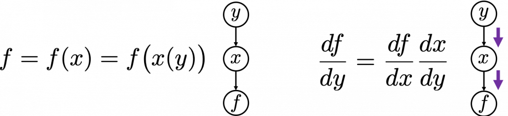
First, let’s think about the simplest type of chain rule. Assume that you have a function $f=f(x)=f(x(y))$, and relations of the functions are displayed as the graphical model at the left side of the figure below. Variables are a type of function, so you should think that every node in graphical models denotes a function. Arrows in purple in the right side of the chart show how information propagate in differentiation.

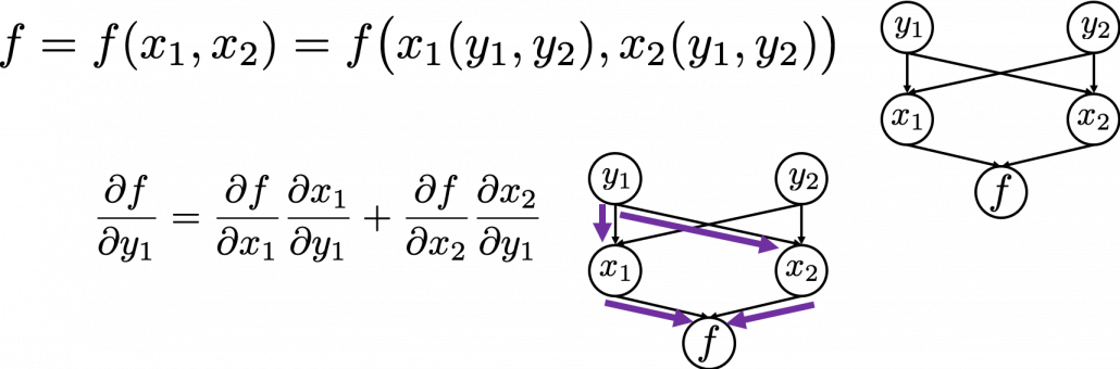
Next, if you a function $f$ , which has two variances  $x_1$ and $x_2$. And both of the variances also share two variances  $y_1$ and $y_2$. When you take partial differentiation of $f$ with respect to $y_1$ or $y_2$, the formula is a little tricky. Let’s think about how to calculate $\frac{\partial f}{\partial y_1}$. The variance $y_1$ propagates to $f$ via $x_1$ and $x_2$. In this case the partial differentiation has two terms as below.

In chain rules, you have to think about all the routes where a variance can propagate through. If you generalize chain rules, that is like below, and you need to understand chain rules in this way to understanding any types of back propagation.

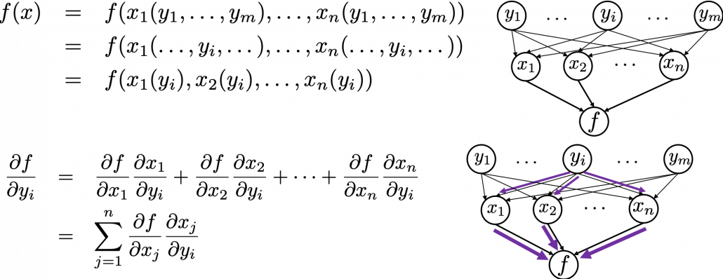
The figure above shows that if you calculate partial differentiation of $f$ with respect to $y_i$, the partial differentiation has $n$ terms in total because $y_i$ propagates to $f$ via $n$ variances.

2, Chain rules in LSTM

I would like you to remember the figure I used to show how errors propagate backward during backprop of simple RNNs. The errors at the last time step propagates only at the last time step.

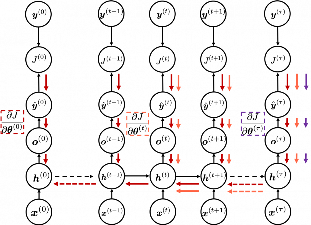
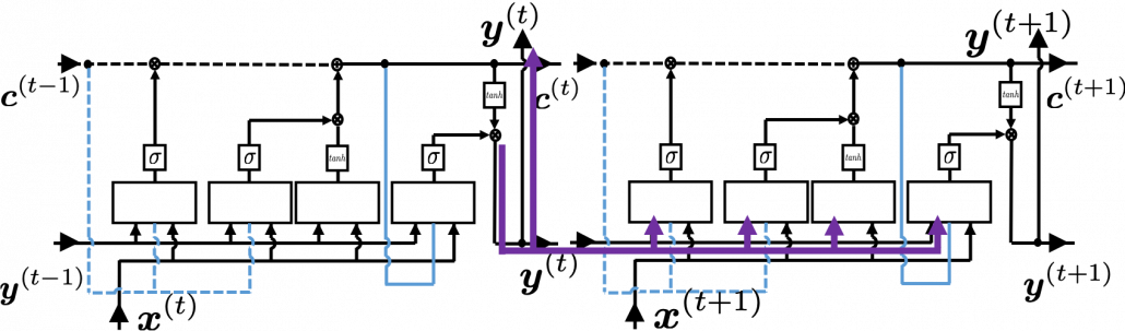
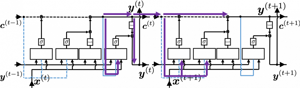
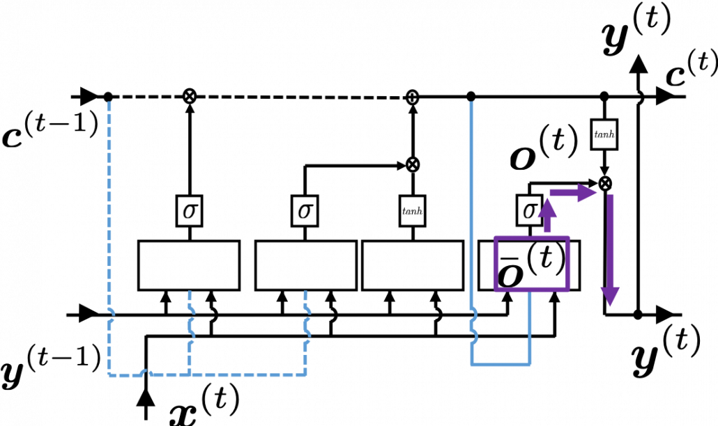
At RNN block level, the flows of errors are the same in LSTM backprop, but the flow of errors in each block is much more complicated in LSTM backprop.

3, How LSTMs tackle exploding/vanishing gradients problems

LSTMs do not solve, vanishing gradient problems, but instead they mitigate vanishing/exploding gradient problems.

Yasuto Tamura

Data Science Intern at DATANOMIQ. Majoring in computer science. Currently studying mathematical sides of deep learning, such as densely connected layers, CNN, RNN, autoencoders, and making study materials on them. Also started aiming at Bayesian deep learning algorithms.