Deep Learning – Data Science Blog

Understanding LSTM forward propagation in two ways

August 31, 2020/0 Comments/in Artificial Intelligence, Data Mining, Data Science, Data Science Hack, Deep Learning, Machine Learning, Main Category, Predictive Analytics /by Yasuto Tamura

*This article is only for the sake of understanding the equations in the second page of the paper named “LSTM: A Search Space Odyssey”. If you have no trouble understanding the equations of LSTM forward propagation, I recommend you to skip this article and go the the next article.

1. Preface

I heard that in Western culture, smart people write textbooks so that other normal people can understand difficult stuff, and that is why textbooks in Western countries tend to be bulky, but also they are not so difficult as they look. On the other hand in Asian culture, smart people write puzzling texts on esoteric topics, and normal people have to struggle to understand what noble people wanted to say. Publishers also require the authors to keep the texts as short as possible, so even though the textbooks are thin, usually students have to repeat reading the textbooks several times because usually they are too abstract.

Both styles have cons and pros, and usually I prefer Japanese textbooks because they are concise, and sometimes it is annoying to read Western style long texts with concrete straightforward examples to reach one conclusion. But a problem is that when it comes to explaining LSTM, almost all the text books are like Asian style ones. Every study material seems to skip the proper steps necessary for “normal people” to understand its algorithms. But after actually making concrete slides on mathematics on LSTM, I understood why: if you write down all the equations on LSTM forward/back propagation, that is going to be massive, and actually I had to make 100-page PowerPoint animated slides to make it understandable to people like me.

I already had a feeling that “Does it help to understand only LSTM with this precision? I should do more practical codings.” For example François Chollet, the developer of Keras, in his book, said as below.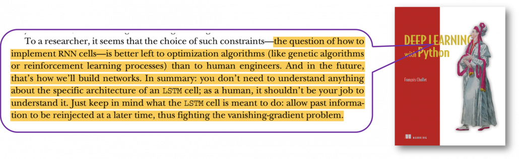

For me that sounds like “We have already implemented RNNs for you, so just shut up and use Tensorflow/Keras.” Indeed, I have never cared about the architecture of my Mac Book Air, but I just use it every day, so I think he is to the point. To make matters worse, for me, a promising algorithm called Transformer seems to be replacing the position of LSTM in natural language processing. But in this article series and in my PowerPoint slides, I tried to explain as much as possible, contrary to his advice.

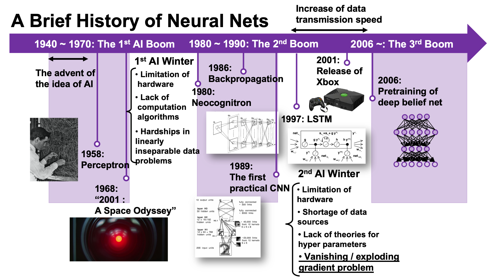
But I think, or rather hope, it is still meaningful to understand this 23-year-old algorithm, which is as old as me. I think LSTM did build a generation of algorithms for sequence data, and actually Sepp Hochreiter, the inventor of LSTM, has received Neural Network Pioneer Award 2021 for his work.

I hope those who study sequence data processing in the future would come to this article series, and study basics of RNN just as I also study classical machine learning algorithms.

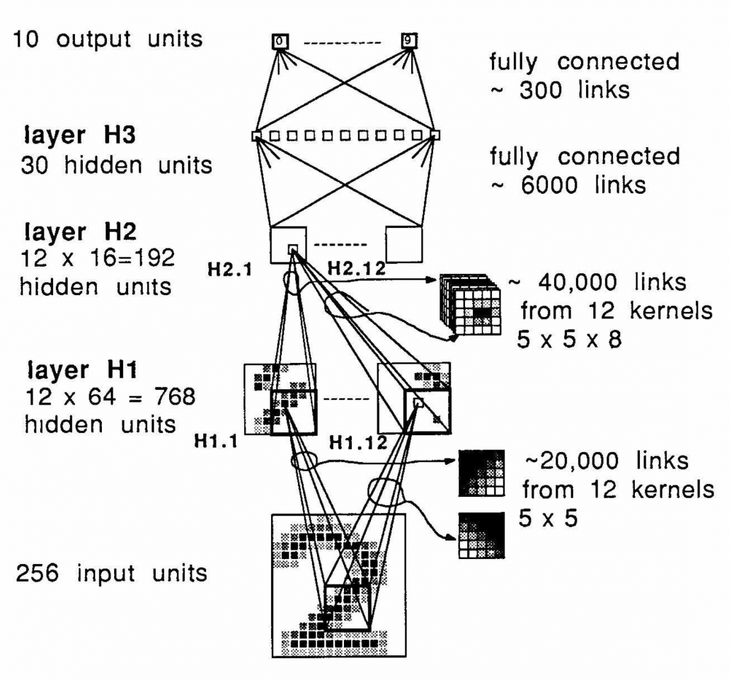
*In this article “Densely Connected Layers” is written as “DCL,” and “Convolutional Neural Network” as “CNN.”

2. Why LSTM?

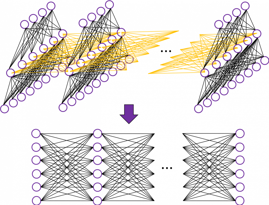
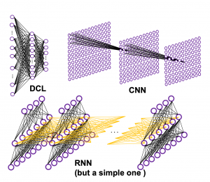
First of all, let’s take a brief look at what I said about the structures of RNNs, in the first and the second article. A simple RNN is basically densely connected network with a few layers. But the RNN gets an input every time step, and it gives out an output at the time step. Part of information in the middle layer are succeeded to the next time step, and in the next time step, the RNN also gets an input and gives out an output. Therefore, virtually a simple RNN behaves almost the same way as densely connected layers with many layers during forward/back propagation if you focus on its recurrent connections.

That is why simple RNNs suffer from vanishing/exploding gradient problems, where the information exponentially vanishes or explodes when its gradients are multiplied many times through many layers during back propagation. To be exact, I think you need to consider this problem precisely like you can see in this paper. But for now, please at least keep it in mind that when you calculate a gradient of an error function with respect to parameters of simple neural networks, you have to multiply parameters many times like below, and this type of calculation usually leads to vanishing/exploding gradient problem.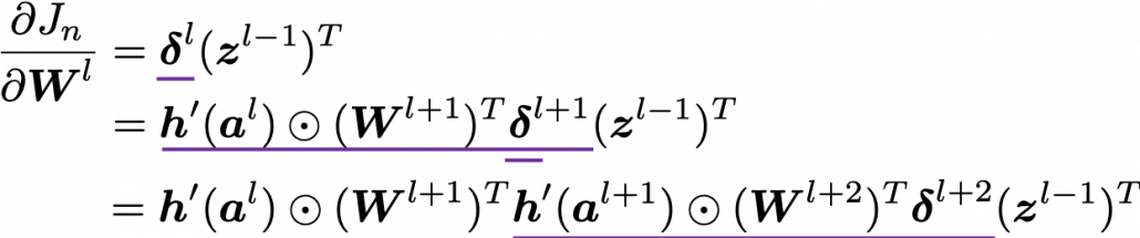

LSTM was invented as a way to tackle such problems as I mentioned in the last article.

3. How to display LSTM

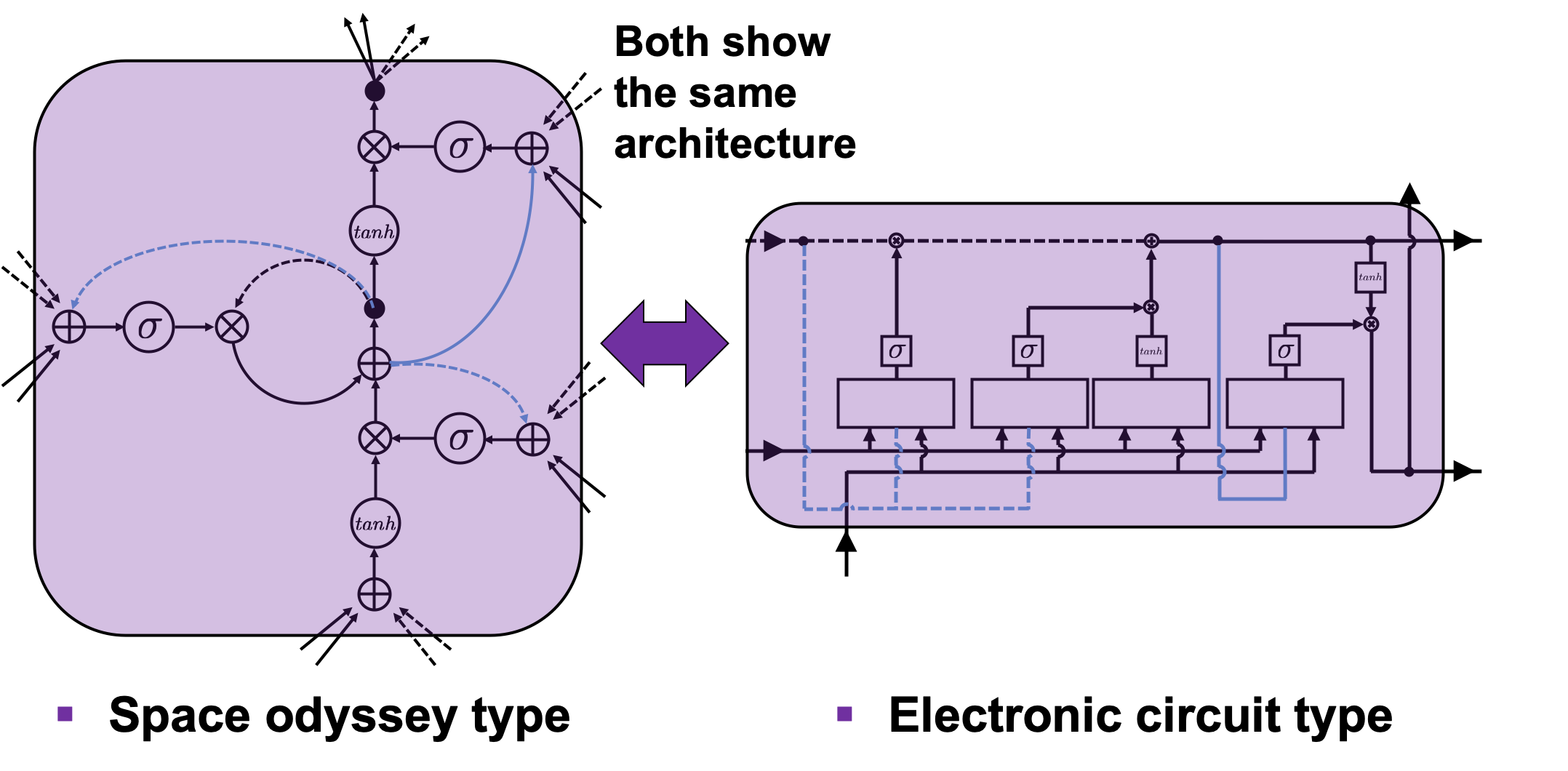
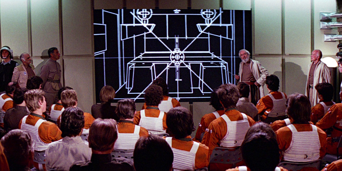
I would like you to just go to image search on Google, Bing, or Yahoo!, and type in “LSTM.” I think you will find many figures, but basically LSTM charts are roughly classified into two types: in this article I call them “Space Odyssey type” and “electronic circuit type”, and in conclusion, I highly recommend you to understand LSTM as the “electronic circuit type.”

*I just randomly came up with the terms “Space Odyssey type” and “electronic circuit type” because the former one is used in the paper I mentioned, and the latter one looks like an electronic circuit to me. You do not have to take how I call them seriously.

However, not that all the well-made explanations on LSTM use the “electronic circuit type,” and I am sure you sometimes have to understand LSTM as the “space odyssey type.” And the paper “LSTM: A Search Space Odyssey,” which I learned a lot about LSTM from, also adopts the “Space Odyssey type.”

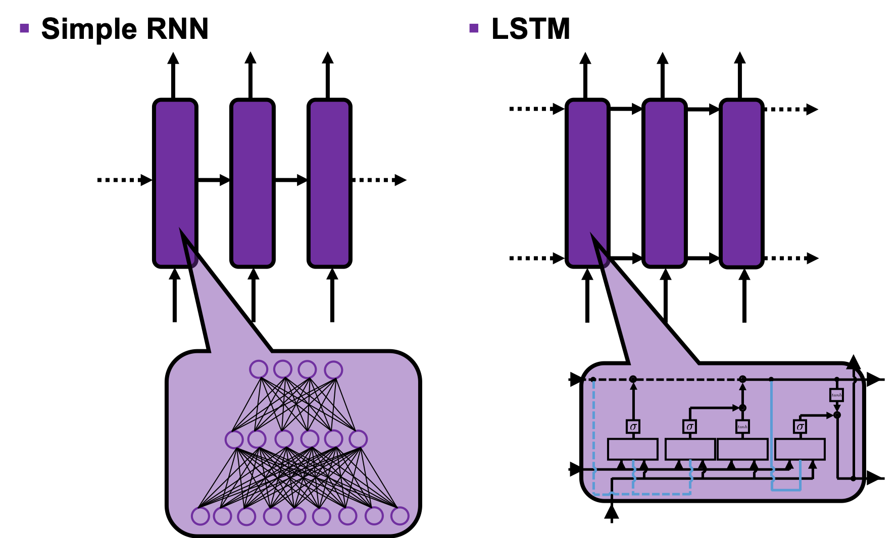
The main reason why I recommend the “electronic circuit type” is that its behaviors look closer to that of simple RNNs, which you would have seen if you read my former articles.

*Behaviors of both of them look different, but of course they are doing the same things.

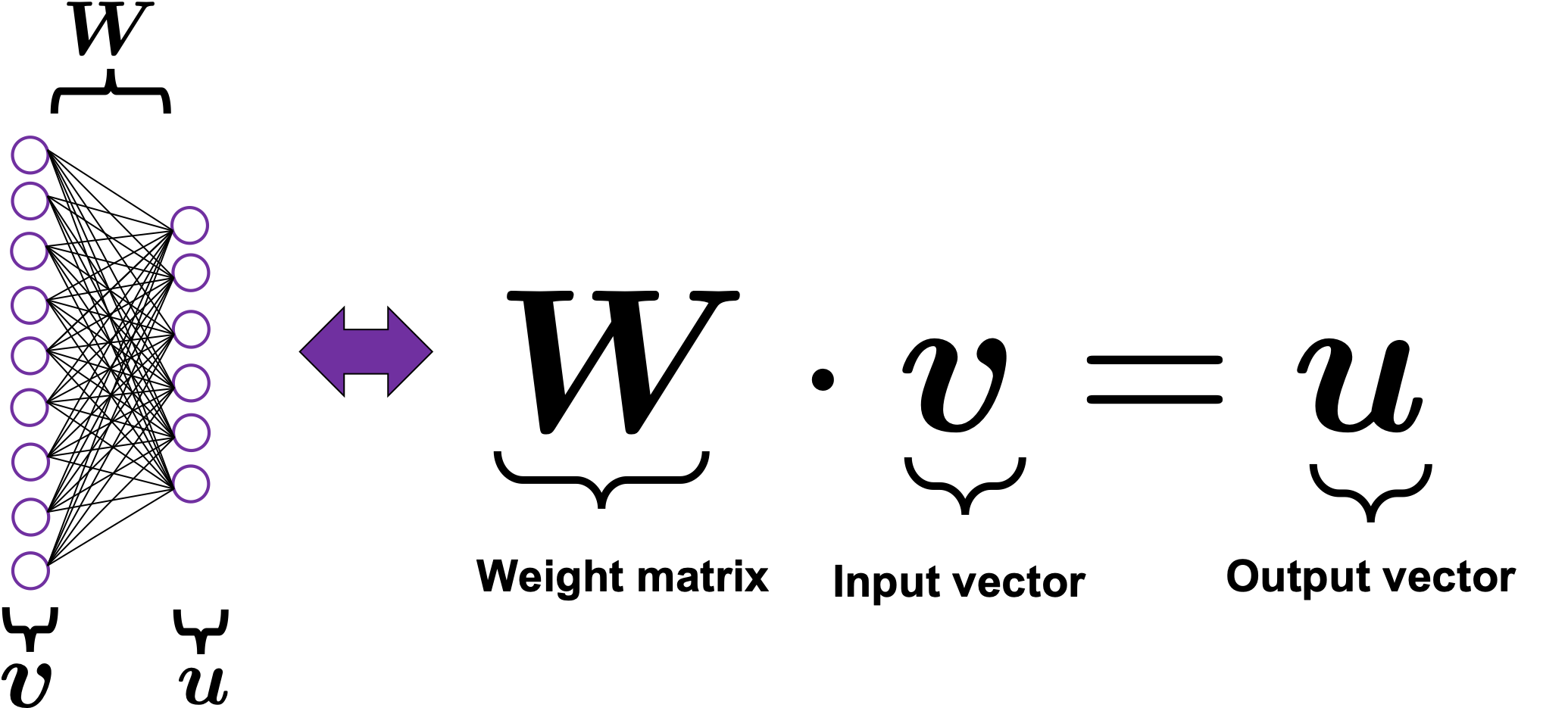
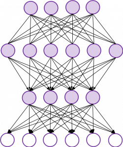
If you have some understanding on DCL, I think it was not so hard to understand how simple RNNs work because simple RNNs are mainly composed of linear connections of neurons and weights, whose structures are the same almost everywhere. And basically they had only straightforward linear connections as you can see below.

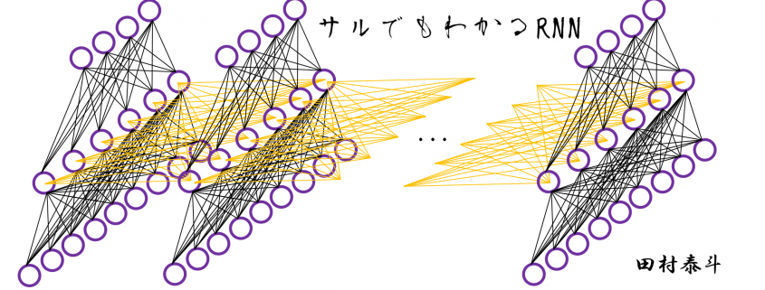
But from now on, I would like you to give up the ideas that LSTM is composed of connections of neurons like the head image of this article series. If you do that, I think that would be chaotic and I do not want to make a figure of it on Power Point. In short, sooner or later you have to understand equations of LSTM.

4. Forward propagation of LSTM in “electronic circuit type”

*For further understanding of mathematics of LSTM forward/back propagation, I recommend you to download my slides.

The behaviors of an LSTM block is quite similar to that of a simple RNN block: an RNN block gets an input every time step and gets information from the RNN block of the last time step, via recurrent connections. And the block succeeds information to the next block.

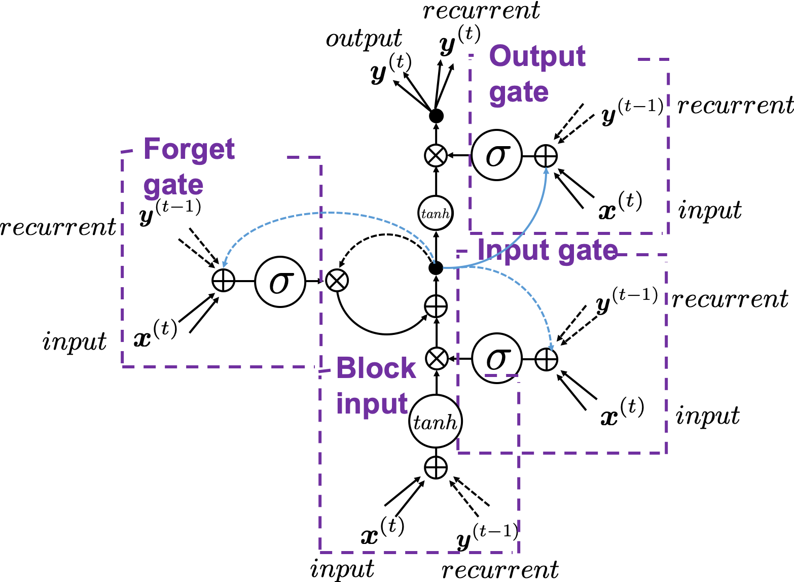
Let’s look at the simplified architecture of an LSTM block. First of all, you should keep it in mind that LSTM have two streams of information: the one going through all the gates, and the one going through cell connections, the “highway” of LSTM block. For simplicity, we will see the architecture of an LSTM block without peephole connections, the lines in blue. The flow of information through cell connections is relatively uninterrupted. This helps LSTMs to retain information for a long time.

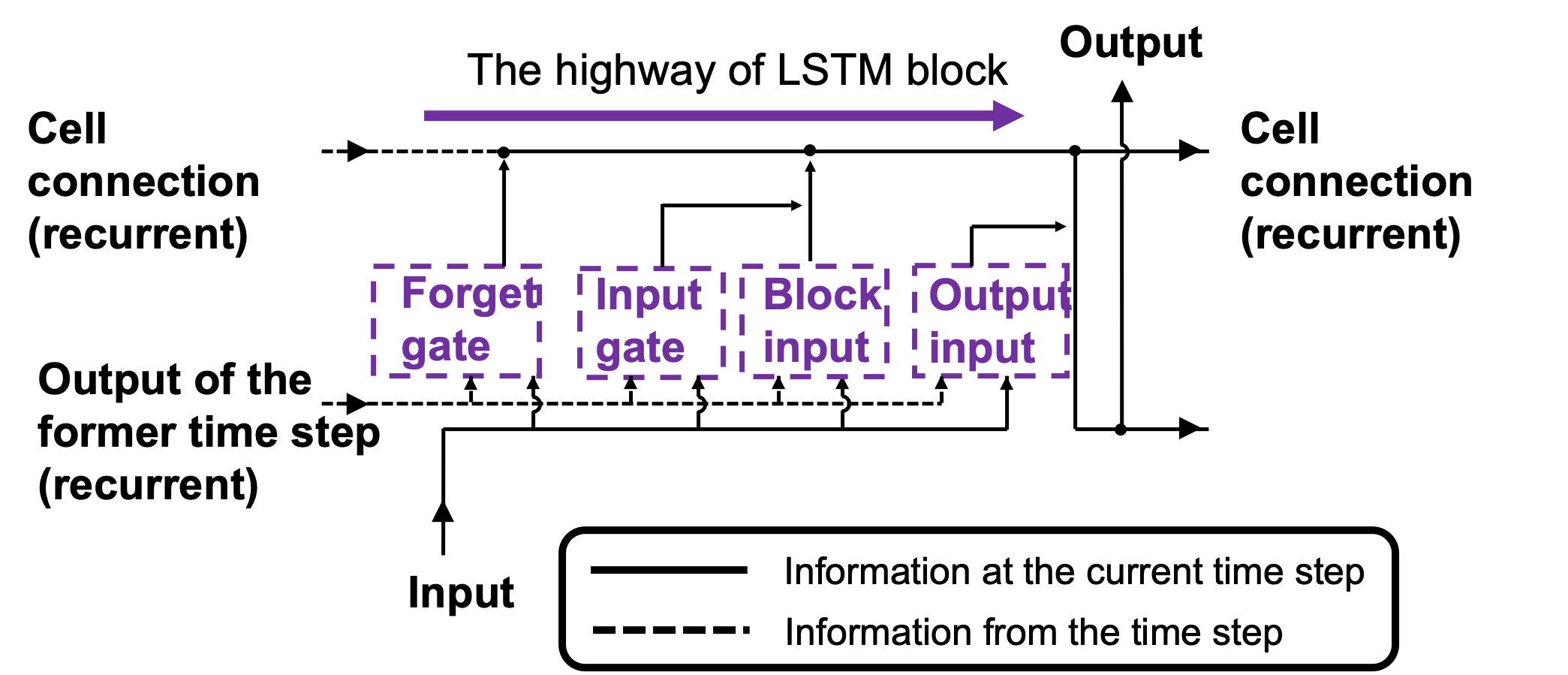
In a LSTM block, the input and the output of the former time step separately go through sections named “gates”: input gate, forget gate, output gate, and block input. The outputs of the forget gate, the input gate, and the block input join the highway of cell connections to renew the value of the cell.

*The small two dots on the cell connections are the “on-ramp” of cell conection highway.

*You would see the terms “input gate,” “forget gate,” “output gate” almost everywhere, but how to call the “block gate” depends on textbooks.

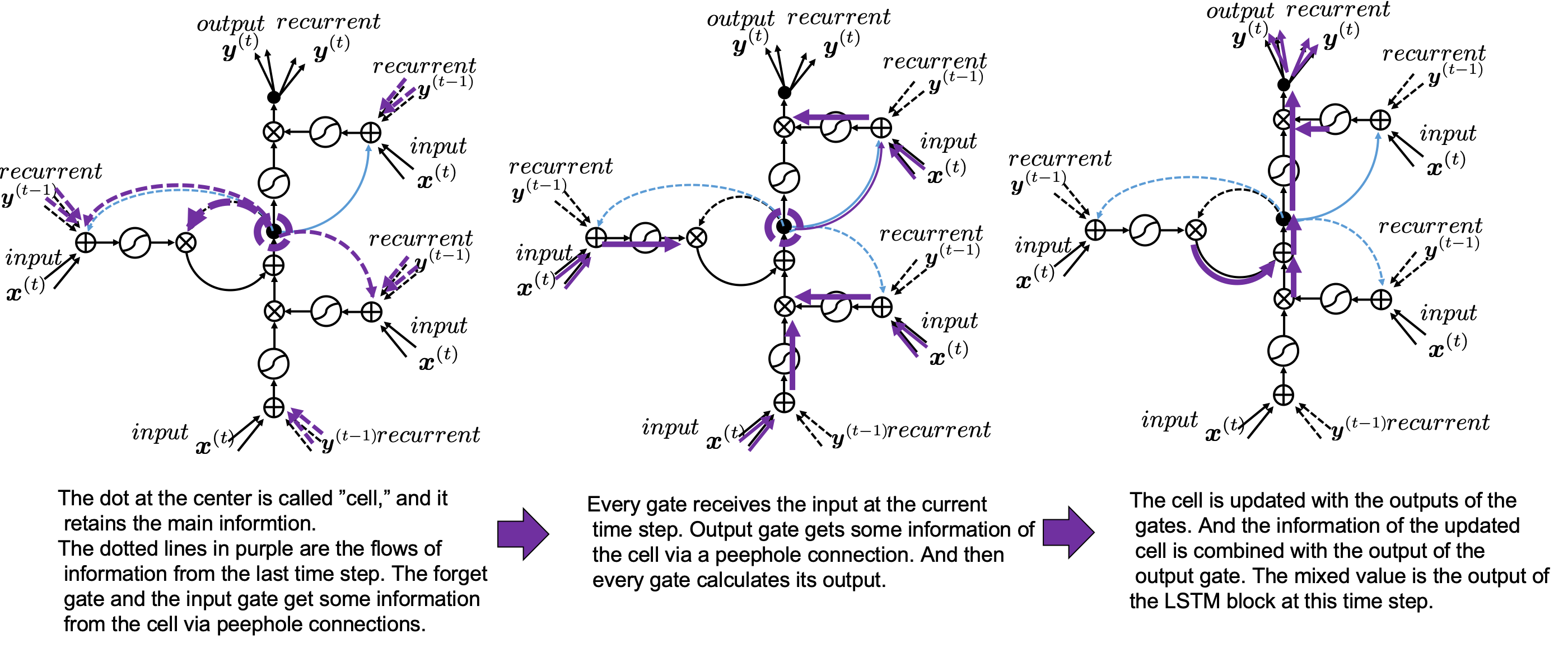
Let’s look at the structure of an LSTM block a bit more concretely. An LSTM block at the time step $(t)$ gets $\boldsymbol{y}^{(t-1)}$ , the output at the last time step, and $\boldsymbol{c}^{(t-1)}$ , the information of the cell at the time step $(t-1)$ , via recurrent connections. The block at time step $(t)$ gets the input $\boldsymbol{x}^{(t)}$ , and it separately goes through each gate, together with $\boldsymbol{y}^{(t-1)}$ . After some calculations and activation, each gate gives out an output. The outputs of the forget gate, the input gate, the block input, and the output gate are respectively $\boldsymbol{f}^{(t)}, \boldsymbol{i}^{(t)}, \boldsymbol{z}^{(t)}, \boldsymbol{o}^{(t)}$ . The outputs of the gates are mixed with $\boldsymbol{c}^{(t-1)}$ and the LSTM block gives out an output $\boldsymbol{y}^{(t)}$ , and gives $\boldsymbol{y}^{(t)}$ and $\boldsymbol{c}^{(t)}$ to the next LSTM block via recurrent connections.

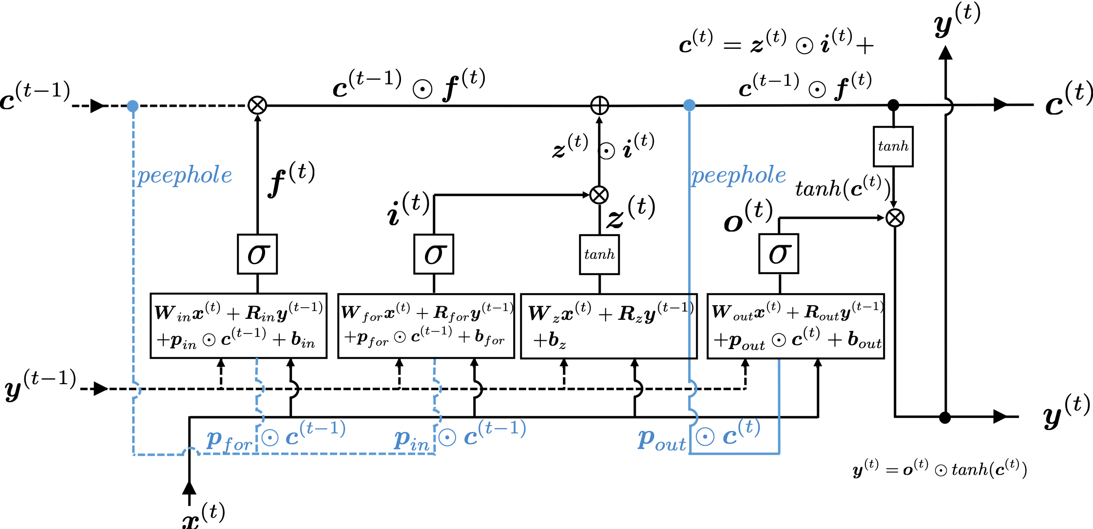
You calculate $\boldsymbol{f}^{(t)}, \boldsymbol{i}^{(t)}, \boldsymbol{z}^{(t)}, \boldsymbol{o}^{(t)}$ as below.

$\boldsymbol{f}^{(t)}= \sigma(\boldsymbol{W}_{for} \boldsymbol{x}^{(t)} + \boldsymbol{R}_{for} \boldsymbol{y}^{(t-1)} + \boldsymbol{b}_{for})$
$\boldsymbol{i}^{(t)}=\sigma(\boldsymbol{W}_{in} \boldsymbol{x}^{(t)} + \boldsymbol{R}_{in} \boldsymbol{y}^{(t-1)} + \boldsymbol{b}_{in})$
$\boldsymbol{z}^{(t)}=tanh(\boldsymbol{W}_z \boldsymbol{x}^{(t)} + \boldsymbol{R}_z \boldsymbol{y}^{(t-1)} + \boldsymbol{b}_z)$
$\boldsymbol{o}^{(t)}=\sigma(\boldsymbol{W}_{out} \boldsymbol{x}^{(t)} + \boldsymbol{R}_{out} \boldsymbol{y}^{(t-1)} + \boldsymbol{b}_{out})$

*You have to keep it in mind that the equations above do not include peephole connections, which I am going to show with blue lines in the end.

The equations above are quite straightforward if you understand forward propagation of simple neural networks. You add linear products of $\boldsymbol{y}^{(t)}$ and $\boldsymbol{c}^{(t)}$ with different weights in each gate. What makes LSTMs different from simple RNNs is how to mix the outputs of the gates with the cell connections. In order to explain that, I need to introduce a mathematical operator called Hadamard product, which you denote as $\odot$ . This is a very simple operator. This operator produces an elementwise product of two vectors or matrices with identical shape.

With this Hadamar product operator, the renewed cell and the output are calculated as below.

$\boldsymbol{c}^{(t)} = \boldsymbol{z}^{(t)}\odot \boldsymbol{i}^{(t)} + \boldsymbol{c}^{(t-1)} \odot \boldsymbol{f}^{(t)}$
$\boldsymbol{y}^{(t)} = \boldsymbol{o}^{(t)} \odot tanh(\boldsymbol{c}^{(t)})$

The values of $\boldsymbol{f}^{(t)}, \boldsymbol{i}^{(t)}, \boldsymbol{z}^{(t)}, \boldsymbol{o}^{(t)}$ are compressed into the range of $[0, 1]$ or $[-1, 1]$ with activation functions. You can see that the input gate and the block input give new information to the cell. The part $\boldsymbol{c}^{(t-1)} \odot \boldsymbol{f}^{(t)}$ means that the output of the forget gate “forgets” the cell of the last time step by multiplying the values from 0 to 1 elementwise. And the cell $\boldsymbol{c}^{(t)}$ is activated with $tanh()$ and the output of the output gate “suppress” the activated value of $\boldsymbol{c}^{(t)}$ . In other words, the output gatedecides how much information to give out as an output of the LSTM block. The output of every gate depends on the input $\boldsymbol{x}^{(t)}$ , and the recurrent connection $\boldsymbol{y}^{(t-1)}$ . That means an LSTM block learns to forget the cell of the last time step, to renew the cell, and to suppress the output. To describe in an extreme manner, if all the outputs of every gate are always $(1, 1, …1)^T$ , LSTMs forget nothing, retain information of inputs at every time step, and gives out everything. And if all the outputs of every gate are always $(0, 0, …0)^T$ , LSTMs forget everything, receive no inputs, and give out nothing.

This model has one problem: the outputs of each gate do not directly depend on the information in the cell. To solve this problem, some LSTM models introduce some flows of information from the cell to each gate, which are shown as lines in blue in the figure below.

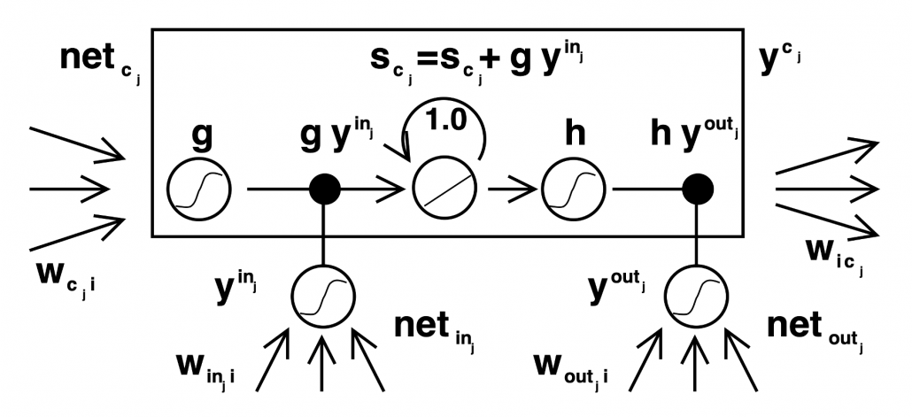
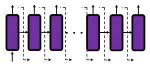
LSTM models, for example the one with or without peephole connection, depend on the library you use, and the model I have showed is one of standard LSTM structure. However no matter how complicated structure of an LSTM block looks, you usually cover it with a black box as below and show its behavior in a very simplified way.

5. Space Odyssey type

I personally think there is no advantages of understanding how LSTMs work with this Space Odyssey type chart, but in several cases you would have to use this type of chart. So I will briefly explain how to look at that type of chart, based on understandings of LSTMs you have gained through this article.

In Space Odyssey type of LSTM chart, at the center is a cell. Electronic circuit type of chart, which shows the flow of information of the cell as an uninterrupted “highway” in an LSTM block. On the other hand, in a Spacey Odyssey type of chart, the information of the cell rotate at the center. And each gate gets the information of the cell through peephole connections, $\boldsymbol{x}^{(t)}$ , the input at the time step $(t)$ , sand $\boldsymbol{y}^{(t-1)}$ , the output at the last time step $(t-1)$ , which came through recurrent connections. In Space Odyssey type of chart, you can more clearly see that the information of the cell go to each gate through the peephole connections in blue. Each gate calculates its output.

Just as the charts you have seen, the dotted line denote the information from the past. First, the information of the cell at the time step $(t-1)$ goes to the forget gate and get mixed with the output of the forget cell In this process the cell is partly “forgotten.” Next, the input gate and the block input are mixed to generate part of new value of the the cell at time step $(t)$ . And the partly “forgotten” $\boldsymbol{c}^{(t-1)}$ goes back to the center of the block and it is mixed with the output of the input gate and the block input. That is how $\boldsymbol{c}^{(t)}$ is renewed. And the value of new cell flow to the top of the chart, being mixed with the output of the output gate. Or you can also say the information of new cell is “suppressed” with the output gate.

I have finished the first four articles of this article series, and finally I am gong to write about back propagation of LSTM in the next article. I have to say what I have written so far is all for the next article, and my long long Power Point slides.

[References]

[1] Klaus Greff, Rupesh Kumar Srivastava, Jan Koutník, Bas R. Steunebrink, Jürgen Schmidhuber, “LSTM: A Search Space Odyssey,” (2017)

[2] Francois Chollet, Deep Learning with Python,(2018), Manning , pp. 202-204

[3] “Sepp Hochreiter receives IEEE CIS Neural Networks Pioneer Award 2021”, Institute of advanced research in artificial intelligence, (2020)
URL: https://www.iarai.ac.at/news/sepp-hochreiter-receives-ieee-cis-neural-networks-pioneer-award-2021/?fbclid=IwAR27cwT5MfCw4Tqzs3MX_W9eahYDcIFuoGymATDR1A-gbtVmDpb8ExfQ87A

[4] Oketani Takayuki, “Machine Learning Professional Series: Deep Learning,” (2015), pp. 120-125
岡谷貴之著, 「機械学習プロフェッショナルシリーズ深層学習」, (2015), pp. 120-125

[5] Harada Tatsuya, “Machine Learning Professional Series: Image Recognition,” (2017), pp. 252-257
原田達也著, 「機械学習プロフェッショナルシリーズ画像認識」, (2017), pp. 252-257

[6] “Understandable LSTM ~ With the Current Trends,” Qiita, (2015)
「わかるLSTM ～最近の動向と共に」, Qiita, (2015)
URL: https://qiita.com/t_Signull/items/21b82be280b46f467d1b

A brief history of neural nets: everything you should know before learning LSTM

July 16, 2020/0 Comments/in Artificial Intelligence, Data Mining, Data Science, Data Science Hack, Deep Learning, Machine Learning, Main Category, Predictive Analytics, TensorFlow /by Yasuto Tamura

This series is not a college course or something on deep learning with strict deadlines for assignments, so let’s take a detour from practical stuff and take a brief look at the history of neural networks.

The history of neural networks is also a big topic, which could be so long that I had to prepare another article series. And usually I am supposed to begin such articles with something like “The term ‘AI’ was first used by John McCarthy in Dartmouth conference 1956…” but you can find many of such texts written by people with much more experiences in this field. Therefore I am going to write this article from my point of view, as an intern writing articles on RNN, as a movie buff, and as one of many Japanese men who spent a great deal of childhood with video games.

We are now in the third AI boom, and some researchers say this boom began in 2006. A professor in my university said there we are now in a kind of bubble economy in machine learning/data science industry, but people used to say “Stop daydreaming” to AI researchers. The second AI winter is partly due to vanishing/exploding gradient problem of deep learning. And LSTM was invented as one way to tackle such problems, in 1997.

1, First AI boom

In the first AI boom, I think people were literally “daydreaming.” Even though the applications of machine learning algorithms were limited to simple tasks like playing chess, checker, or searching route of 2d mazes, and sometimes this time is called GOFAI (Good Old Fashioned AI).

Source: https://www.youtube.com/watch?v=K-HfpsHPmvw&feature=youtu.be

Even today when someone use the term “AI” merely for tasks with neural networks, that amuses me because for me deep learning is just statistically and automatically training neural networks, which are capable of universal approximation, into some classifiers/regressors. Actually the algorithms behind that is quite impressive, but the structure of human brains is much more complicated. The hype of “AI” already started in this first AI boom. Let me take an example of machine translation in this video. In fact the research of machine translation already started in the early 1950s, and of specific interest in the time was translation between English and Russian due to Cold War. In the first article of this series, I said one of the most famous applications of RNN is machine translation, such as Google Translation, DeepL. They are a type of machine translation called neural machine translation because they use neural networks, especially RNNs. Neural machine translation was an astonishing breakthrough around 2014 in machine translation field. The former major type of machine translation was statistical machine translation, based on statistical language models. And the machine translator in the first AI boom was rule base machine translators, which are more primitive than statistical ones.

Source: https://news.cornell.edu/stories/2019/09/professors-perceptron-paved-way-ai-60-years-too-soon

The most remarkable invention in this time was of course perceptron by Frank Rosenblatt. Some people say that this is the first neural network. Even though you can implement perceptron with a-few-line codes in Python, obviously they did not have Jupyter Notebook in those days. The perceptron was implemented as a huge instrument named Mark 1 Perceptron, and it was composed of randomly connected wires. I do not precisely know how it works, but it was a huge effort to implement even the most primitive type of neural networks. They needed to use a big lighting fixture to get a 20*20 pixel image using 20*20 array of cadmium sulphide photocells. The research by Rosenblatt, however, was criticized by Marvin Minsky in his book because perceptrons could only be used for linearly separable data. To make matters worse the criticism prevailed as that more general, multi-layer perceptrons were also not useful for linearly inseparable data (as I mentioned in the first article, multi-layer perceptrons, namely normal neural networks, can be universal approximators, which have potentials to classify/regress various types of complex data). In case you do not know what “linearly separable” means, imagine that there are data plotted on a piece of paper. If an elementary school kid can draw a border line between two clusters of the data with a ruler and a pencil on the paper, the 2d data is “linearly separable”….

With big disappointments to the research on “electronic brains,” the budget of AI research was reduced and AI research entered its first winter.

Source: https://www.nzz.ch/digital/ehre-fuer-die-deep-learning-mafia-ld.1472761?reduced=true and https://anatomiesofintelligence.github.io/posts/2019-06-21-organization-mark-i-perceptron

I think the frame problem(1969), by John McCarthy and Patrick J. Hayes, is also an iconic theory in the end of the first AI boom. This theory is known as a story of creating a robot trying to pull out its battery on a wheeled wagon in a room. The first prototype of the robot, named R1, naively tried to pull out the wagon form the room, and the bomb exploded. The problems was obvious: R1 was not programmed to consider the risks by taking each action, so the researchers made the next prototype named R1D1, which was programmed to consider the potential risks of taking each action. When R1D1 tried to pull out the wagon, it realized the risk of pulling the bomb together with the battery. But soon it started considering all the potential risks, such as the risk of the ceiling falling down, the distance between the wagon and all the walls, and so on, when the bomb exploded. The next problem was also obvious: R1D1 was not programmed to distinguish if the factors are relevant of irrelevant to the main purpose, and the next prototype R2D1 was programmed to do distinguish them. This time, R2D1 started thinking about “whether the factor is irrelevant to the main purpose,” on every factor measured, and again the bomb exploded. How can we get a perfect AI, R2D2?

The situation of mentioned above is a bit extreme, but it is said AI could also get stuck when it try to take some super simple actions like finding a number in a phone book and make a phone call. It is difficult for an artificial intelligence to decide what is relevant and what is irrelevant, but humans will not get stuck with such simple stuff, and sometimes the frame problem is counted as the most difficult and essential problem of developing AI. But personally I think the original frame problem was unreasonable in that McCarthy, in his attempts to model the real world, was inflexible in his handling of the various equations involved, treating them all with equal weight regardless of the particular circumstances of a situation. Some people say that McCarthy, who was an advocate for AI, also wanted to see the field come to an end, due to its failure to meet the high expectations it once aroused.

Not only the frame problem, but also many other AI-related technological/philosophical problems have been proposed, such as Chinese room (1980), the symbol grounding problem (1990), and they are thought to be as hardships in inventing artificial intelligence, but I omit those topics in this article.

*The name R2D2 did not come from the famous story of frame problem. The story was Daniel Dennett first proposed the story of R2D2 in his paper published in 1984. Star Wars was first released in 1977. It is said that the name R2D2 came from “Reel 2, Dialogue 2,” which George Lucas said while film shooting. And the design of C3PO came from Maria in Metropolis(1927). It is said that the most famous AI duo in movie history was inspired by Tahei and Matashichi in The Hidden Fortress(1958), directed by Kurosawa Akira.

Source: https://criterioncollection.tumblr.com/post/135392444906/the-original-r2-d2-and-c-3po-the-hidden-fortress

Interestingly, in the end of the first AI boom, 2001: A Space Odyssey, directed by Stanley Kubrick, was released in 1968. Unlike conventional fantasylike AI characters, for example Maria in Metropolis(1927), HAL 9000 was portrayed as a very realistic AI, and the movie already pointed out the risk of AI being insane when it gets some commands from several users. HAL 9000 still has been a very iconic character in AI field. For example when you say some quotes from 2001: A Space Odyssey to Siri you get some parody responses. I also thin you should keep it in mind that in order to make an AI like HAL 9000 come true, for now RNNs would be indispensable in many ways: you would need RNNs for better voice recognition, better conversational system, and for reading lips.

Source: https://imgflip.com/memetemplate/34339860/Open-the-pod-bay-doors-Hal

*Just as you cannot understand Monty Python references in Python official tutorials without watching Monty Python and the Holy Grail, you cannot understand many parodies in AI contexts without watching 2001: A Space Odyssey. Even though the movie had some interview videos with some researchers and some narrations, Stanley Kubrick cut off all the footage and made the movie very difficult to understand. Most people did not or do not understand that it is a movie about aliens who gave homework of coming to Jupiter to human beings.

2, Second AI boom/winter

Source: Fukushima Kunihiko, “Neocognitron: A self-organizing neural network model for a mechanism of pattern recognition unaffected by shift in position,” (1980)

I am not going to write about the second AI boom in detail, but at least you should keep it in mind that convolutional neural network(CNN) is a keyword in this time. Neocognitron, an artificial model of how sight nerves perceive thing, was invented by Kunihiko Fukushima in 1980, and the model is said to be the origin on CNN. And Neocognitron got inspired by the Hubel and Wiesel’s research on sight nerves. In 1989, a group in AT & T Bell Laboratory led by Yann LeCun invented the first practical CNN to read handwritten digit.

Y. LeCun, “Backpropagation Applied to Handwritten Zip Code Recognition,” (1989)

Another turning point in this second AI boom was that back propagation algorithm was discovered, and the CNN by LeCun was also trained with back propagation. LeCun made a deep neural networks with some layers in 1998 for more practical uses.

But his research did not gain so much attention like today, because AI research entered its second winter at the beginning of the 1990s, and that was partly due to vanishing/exploding gradient problem of deep learning. People knew that neural networks had potentials of universal approximation, but when they tried to train naively stacked neural nets, the gradients, which you need for training neural networks, exponentially increased/decreased. Even though the CNN made by LeCun was the first successful case of “deep” neural nets which did not suffer from the vanishing/exploding gradient problem so much, deep learning research also stagnated in this time.

The ultimate goal of this article series is to understand LSTM at a more abstract/mathematical level because it is one of the practical RNNs, but the idea of LSTM (Long Short Term Memory) itself was already proposed in 1997 as an RNN algorithm to tackle vanishing gradient problem. (Exploding gradient problem is solved with a technique named gradient clipping, and this is easier than techniques for preventing vanishing gradient problems. I am also going to explain it in the next article.) After that some other techniques like introducing forget gate, peephole connections, were discovered, but basically it took some 20 years till LSTM got attentions like today. The reasons for that is lack of hardware and data sets, and that was also major reasons for the second AI winter.

Source: Sepp HochreiterJürgen, Schmidhuber, “Long Short-term Memory,” (1997)

In the 1990s, the mid of second AI winter, the Internet started prevailing for commercial uses. I think one of the iconic events in this time was the source codes WWW(World Wide Web) were announced in 1993. Some of you might still remember that you little by little became able to transmit more data online in this time. That means people came to get more and more access to various datasets in those days, which is indispensable for machine learning tasks.

After all, we could not get HAL 9000 by the end of 2001, but instead we got Xbox console.

3, Video game industry and GPU

Even though research on neural networks stagnated in the 1990s the same period witnessed an advance in the computation of massive parallel linear transformations, due to their need in fields such as image processing.

Computer graphics move or rotate in 3d spaces, and that is also linear transformations. When you think about a car moving in a city, it is convenient to place the car, buildings, and other objects on a fixed 3d space. But when you need to make computer graphics of scenes of the city from a view point inside the car, you put a moving origin point in the car and see the city. The spatial information of the city is calculated as vectors from the moving origin point. Of course this is also linear transformations. Of course I am not talking about a dot or simple figures moving in the 3d spaces. Computer graphics are composed of numerous plane panels, and each of them have at least three vertexes, and they move on 3d spaces. Depending on viewpoints, you need project the 3d graphics in 3d spaces on 2d spaces to display the graphics on devices. You need to calculate which part of the panel is projected to which pixel on the display, and that is called rasterization. Plus, in order to get photophotorealistic image, you need to think about how lights from light sources reflect on the panel and projected on the display. And you also have to put some textures on groups of panels. You might also need to change color spaces, which is also linear transformations.

My point is, in short, you really need to do numerous linear transformations in parallel in image processing.

When it comes to the use of CGI in movies, two pioneer movies were released during this time: Jurassic Park in 1993, and Toy Story in 1995. It is famous that Pixar used to be one of the departments in ILM(Industrial Light and Magic), founded by George Lucas, and Steve Jobs bought the department. Even though the members in Pixar had not even made a long feature film in their lives, after trial and errors, they made the first CGI animated feature movie. On the other hand, in order to acquire funds for the production of Schindler’s List(1993), Steven Spielberg took on Jurassic Park(1993), consequently changing the history of CGI through this “side job.”

Source: http://renderstory.com/jurassic-park-23-years-later/

*I think you have realized that George Lucas is mentioned almost everywhere in this article. His influences on technologies are not only limited to image processing, but also sound measuring system, nonlinear editing system. Photoshop was also originally developed under his company. I need another article series for this topic, but maybe not in Data Science Blog.

Source: https://editorial.rottentomatoes.com/article/5-technical-breakthroughs-in-star-wars-that-changed-movies-forever/

Considering that the first wire-frame computer graphics made and displayed by computers appeared in the scene of displaying the wire frame structure of Death Star in a war room, in Star Wars: A New Hope, the development of CGI was already astonishing at this time. But I think deep learning owe its development more to video game industry.

*I said that the Death Star scene is the first use of graphics made and DISPLAYED by computers, because I have to say one of the first graphics in movie MADE by computer dates back to the legendary title sequence of Vertigo(1958).

When it comes to 3D video games the processing unit has to constantly deal with real time commands from controllers. It is famous that GPU was originally specifically designed for plotting computer graphics. Video game market is the biggest in entertainment industry in general, and it is said that the quality of computer graphics have the strongest correlation with video games sales, therefore enhancing this quality is a priority for the video game console manufacturers.

One good example to see how much video games developed is comparing original Final Fantasy 7 and the remake one. The original one was released in 1997, the same year as when LSTM was invented. And recently the remake version of Final Fantasy 7 was finally released this year. The original one was also made with very big budget, and it was divided into three CD-ROMs. The original one was also very revolutionary given that the former ones of Final Fantasy franchise were all 2d video retro style video games. But still the computer graphics looks like polygons, and in almost all scenes the camera angle was fixed in the original one. On the other hand the remake one is very photorealistic and you can move the angle of the camera as you want while you play the video game.

There were also fierce battles by graphic processor manufacturers in computer video game market in the 1990s, but personally I think the release of Xbox console was a turning point in the development of GPU. To be concrete, Microsoft adopted a type of NV20 GPU for Xbox consoles, and that left some room of programmability for developers. The chief architect of NV20, which was released under the brand of GeForce3, said making major changes in the company’s graphic chips was very risky. But that decision opened up possibilities of uses of GPU beyond computer graphics.

Source: https://de.wikipedia.org/wiki/Nvidia-GeForce-3-Serie

I think that the idea of a programmable GPU provided other scientific fields with more visible benefits after CUDA was launched. And GPU gained its position not only in deep learning, but also many other fields including making super computers.

*When it comes to deep learning, even GPUs have strong rivals. TPU(Tensor Processing Unit) made by Google, is specialized for deep learning tasks, and have astonishing processing speed. And FPGA(Field Programmable Gate Array), which was originally invented customizable electronic circuit, proved to be efficient for reducing electricity consumption of deep learning tasks.

*I am not so sure about this GPU part. Processing unit, including GPU is another big topic, that is beyond my capacity to be honest. I would appreciate it if you could share your view and some references to confirm your opinion, on the comment section or via email.

*If you are interested you should see this video of game fans’ reactions to the announcement of Final Fantasy 7. This is the industry which grew behind the development of deep learning, and many fields where you need parallel computations owe themselves to the nerds who spent a lot of money for video games, including me.

*But ironically the engineers who invented the GPU said they did not play video games simply because they were busy. If you try to study the technologies behind video games, you would not have much time playing them. That is the reality.

We have seen that the in this second AI winter, Internet and GPU laid foundation of the next AI boom. But still the last piece of the puzzle is missing: let’s look at the breakthrough which solved the vanishing /exploding gradient problem of deep learning in the next section.

4, Pretraining of deep belief networks: “The Dawn of Deep Learning”

Some researchers say the invention of pretraining of deep belief network by Geoffrey Hinton was a breakthrough which put an end to the last AI winter. Deep belief networks are different type of networks from the neural networks we have discussed, but their architectures are similar to those of the neural networks. And it was also unknown how to train deep belief nets when they have several layers. Hinton discovered that training the networks layer by layer in advance can tackle vanishing gradient problems. And later it was discovered that you can do pretraining neural networks layer by layer with autoencoders.

*Deep belief network is beyond the scope of this article series. I have to talk about generative models, Boltzmann machine, and some other topics.

The pretraining techniques of neural networks is not mainstream anymore. But I think it is very meaningful to know that major deep learning techniques such as using ReLU activation functions, optimization with Adam, dropout, batch normalization, came up as more effective algorithms for deep learning after the advent of the pretraining techniques, and now we are in the third AI boom.

In the next next article we are finally going to work on LSTM. Specifically, I am going to offer a clearer guide to a well-made paper on LSTM, named “LSTM: A Search Space Odyssey.”

* I make study materials on machine learning, sponsored by DATANOMIQ. I do my best to make my content as straightforward but as precise as possible. I include all of my reference sources. If you notice any mistakes in my materials, including grammatical errors, please let me know (email: yasuto.tamura@datanomiq.de). And if you have any advice for making my materials more understandable to learners, I would appreciate hearing it.

[References]

[1] Taniguchi Tadahiro, “An Illustrated Guide to Artificial Intelligence”, (2010), Kodansha pp. 3-11
谷口忠大著, 「イラストで学ぶ人工知能概論」, (2010), 講談社, pp. 3-11

[2] Francois Chollet, Deep Learning with Python,(2018), Manning , pp. 14-24

[3] Oketani Takayuki, “Machine Learning Professional Series: Deep Learning,” (2015), pp. 1-5, 151-156
岡谷貴之著, 「機械学習プロフェッショナルシリーズ深層学習」, (2015), pp. 1-5, 151-156

[4] Abigail See, Matthew Lamm, “Natural Language Processingwith Deep LearningCS224N/Ling284 Lecture 8:Machine Translation,Sequence-to-sequence and Attention,” (2020),
URL: http://web.stanford.edu/class/cs224n/slides/cs224n-2020-lecture08-nmt.pdf

[5]C. M. Bishop, “Pattern Recognition and Machine Learning,” (2006), Springer, pp. 192-196

[6] Daniel C. Dennett, “Cognitive Wheels: the Frame Problem of AI,” (1984), pp. 1-2

[7] Machiyama Tomohiro, “Understanding Cinemas of 1967-1979,” (2014), Yosensya, pp. 14-30
町山智浩著, 「＜映画の見方＞が分かる本」,(2014), 洋泉社, pp. 14-30

[8] Harada Tatsuya, “Machine Learning Professional Series: Image Recognition,” (2017), pp. 156-157
原田達也著, 「機械学習プロフェッショナルシリーズ画像認識」, (2017), pp. 156-157

[9] Suyama Atsushi, “Machine Learning Professional Series: Bayesian Deep Learning,” (2019)岡谷貴之須山敦志著, 「機械学習プロフェッショナルシリーズベイズ深層学習」, (2019)

[10] “Understandable LSTM ~ With the Current Trends,” Qiita, (2015)
「わかるLSTM ～最近の動向と共に」, Qiita, (2015)
URL: https://qiita.com/t_Signull/items/21b82be280b46f467d1b

[11] Hisa Ando, “WEB+DB PRESS plus series: Technologies Supporting Processors – The World Endlessly Pursuing Speed,” (2017), Gijutsu-hyoron-sya, pp 313-317
Hisa Ando, 「WEB+DB PRESS plusシリーズプロセッサを支える技術― 果てしなくスピードを追求する世界」, (2017), 技術評論社, pp. 313-317

[12] “Takahashi Yoshiki and Utamaru discuss George Lucas,” miyearnZZ Labo, (2016)
“高橋ヨシキと宇多丸　ジョージ・ルーカスを語る,” miyearnZZ Labo, (2016)
URL: https://miyearnzzlabo.com/archives/38865

[13] Katherine Bourzac, “Chip Hall of Fame: Nvidia NV20 The first configurable graphics processor opened the door to a machine-learning revolution,” IEEE SPECTRUM, (2018)
URL: https://spectrum.ieee.org/tech-history/silicon-revolution/chip-hall-of-fame-nvidia-nv20

Data Analytics and Mining for Dummies

July 2, 2020/1 Comment/in Data Mining, Data Science, Deep Learning, Predictive Analytics, Tool Introduction /by Sharma Srishti

Data Analytics and Mining is often perceived as an extremely tricky task cut out for Data Analysts and Data Scientists having a thorough knowledge encompassing several different domains such as mathematics, statistics, computer algorithms and programming. However, there are several tools available today that make it possible for novice programmers or people with no absolutely no algorithmic or programming expertise to carry out Data Analytics and Mining. One such tool which is very powerful and provides a graphical user interface and an assembly of nodes for ETL: Extraction, Transformation, Loading, for modeling, data analysis and visualization without, or with only slight programming is the KNIME Analytics Platform.

KNIME, or the Konstanz Information Miner, was developed by the University of Konstanz and is now popular with a large international community of developers. Initially KNIME was originally made for commercial use but now it is available as an open source software and has been used extensively in pharmaceutical research since 2006 and also a powerful data mining tool for the financial data sector. It is also frequently used in the Business Intelligence (BI) sector.

KNIME as a Data Mining Tool

KNIME is also one of the most well-organized tools which enables various methods of machine learning and data mining to be integrated. It is very effective when we are pre-processing data i.e. extracting, transforming, and loading data.

KNIME has a number of good features like quick deployment and scaling efficiency. It employs an assembly of nodes to pre-process data for analytics and visualization. It is also used for discovering patterns among large volumes of data and transforming data into more polished/actionable information.

Some Features of KNIME:

Free and open source
Graphical and logically designed
Very rich in analytics capabilities
No limitations on data size, memory usage, or functionalities
Compatible with Windows ,OS and Linux
Written in Java and edited with Eclipse.

A node is the smallest design unit in KNIME and each node serves a dedicated task. KNIME contains graphical, drag-drop nodes that require no coding. Nodes are connected with one’s output being another’s input, as a workflow. Therefore end-to-end pipelines can be built requiring no coding effort. This makes KNIME stand out, makes it user-friendly and make it accessible for dummies not from a computer science background.

KNIME workflow designed for graduate admission prediction

KNIME has nodes to carry out Univariate Statistics, Multivariate Statistics, Data Mining, Time Series Analysis, Image Processing, Web Analytics, Text Mining, Network Analysis and Social Media Analysis. The KNIME node repository has a node for every functionality you can possibly think of and need while building a data mining model. One can execute different algorithms such as clustering and classification on a dataset and visualize the results inside the framework itself. It is a framework capable of giving insights on data and the phenomenon that the data represent.

Some commonly used KNIME node groups include:

Input-Output or I/O: Nodes in this group retrieve data from or to write data to external files or data bases.
Data Manipulation: Used for data pre-processing tasks. Contains nodes to filter, group, pivot, bin, normalize, aggregate, join, sample, partition, etc.
Views: This set of nodes permit users to inspect data and analysis results using multiple views. This gives a means for truly interactive exploration of a data set.
Data Mining: In this group, there are nodes that implement certain algorithms (like K-means clustering, Decision Trees, etc.)

Comparison with other tools

The first version of the KNIME Analytics Platform was released in 2006 whereas Weka and R studio were released in 1997 and 1993 respectively. KNIME is a proper data mining tool whereas Weka and R studio are Machine Learning tools which can also do data mining. KNIME integrates with Weka to add machine learning algorithms to the system. The R project adds statistical functionalities as well. Furthermore, KNIME’s range of functions is impressive, with more than 1,000 modules and ready-made application packages. The modules can be further expanded by additional commercial features.

Simple RNN: the first foothold for understanding LSTM

June 17, 2020/0 Comments/in Artificial Intelligence, Data Science, Deep Learning, Machine Learning, Main Category, Mathematics /by Yasuto Tamura

*In this article “Densely Connected Layers” is written as “DCL,” and “Convolutional Neural Network” as “CNN.”

In the last article, I mentioned “When it comes to the structure of RNN, many study materials try to avoid showing that RNNs are also connections of neurons, as well as DCL or CNN.” Even if you manage to understand DCL and CNN, you can be suddenly left behind once you try to understand RNN because it looks like a different field. In the second section of this article, I am going to provide a some helps for more abstract understandings of DCL/CNN , which you need when you read most other study materials.

My explanation on this simple RNN is based on a chapter in a textbook published by Massachusetts Institute of Technology, which is also recommended in some deep learning courses of Stanford University.

First of all, you should keep it in mind that simple RNN are not useful in many cases, mainly because of vanishing/exploding gradient problem, which I am going to explain in the next article. LSTM is one major type of RNN used for tackling those problems. But without clear understanding forward/back propagation of RNN, I think many people would get stuck when they try to understand how LSTM works, especially during its back propagation stage. If you have tried climbing the mountain of understanding LSTM, but found yourself having to retreat back to the foot, I suggest that you read through this article on simple RNNs. It should help you to gain a solid foothold, and you would be ready for trying to climb the mountain again.

*This article is the second article of “A gentle introduction to the tiresome part of understanding RNN.”

1, A brief review on back propagation of DCL.

Simple RNNs are straightforward applications of DCL, but if you do not even have any ideas on DCL forward/back propagation, you will not be able to understand this article. If you more or less understand how back propagation of DCL works, you can skip this first section.

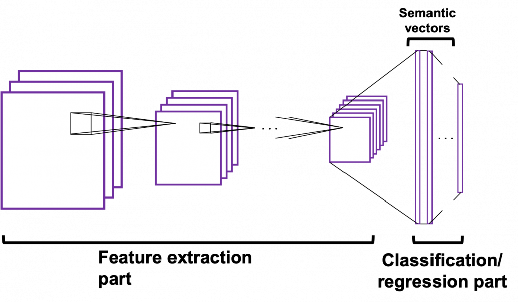
Deep learning is a part of machine learning. And most importantly, whether it is classical machine learning or deep learning, adjusting parameters is what machine learning is all about. Parameters mean elements of functions except for variants. For example when you get a very simple function $f(x)=a + bx + cx^2 + dx^3$ , then $x$ is a variant, and $a, b, c, d$ are parameters. In case of classical machine learning algorithms, the number of those parameters are very limited because they were originally designed manually. Such functions for classical machine learning is useful for features found by humans, after trial and errors(feature engineering is a field of finding such effective features, manually). You adjust those parameters based on how different the outputs(estimated outcome of classification/regression) are from supervising vectors(the data prepared to show ideal answers).

In the last article I said neural networks are just mappings, whose inputs are vectors, matrices, or sequence data. In case of DCLs, inputs are vectors. Then what’s the number of parameters ? The answer depends on the the number of neurons and layers. In the example of DCL at the right side, the number of the connections of the neurons is the number of parameters(Would you like to try to count them? At least I would say “No.”). Unlike classical machine learning you no longer need to do feature engineering, but instead you need to design networks effective for each task and adjust a lot of parameters.

*I think the hype of AI comes from the fact that neural networks find features automatically. But the reality is difficulty of feature engineering was just replaced by difficulty of designing proper neural networks.

It is easy to imagine that you need an efficient way to adjust those parameters, and the method is called back propagation (or just backprop). As long as it is about DCL backprop, you can find a lot of well-made study materials on that, so I am not going to cover that topic precisely in this article series. Simply putting, during back propagation, in order to adjust parameters of a layer you need errors in the next layer. And in order calculate the errors of the next layer, you need errors in the next next layer.

*You should not think too much about what the “errors” exactly mean. Such “errors” are defined in this context, and you will see why you need them if you actually write down all the mathematical equations behind backprops of DCL.

The red arrows in the figure shows how errors of all the neurons in a layer propagate backward to a neuron in last layer. The figure shows only some sets of such errors propagating backward, but in practice you have to think about all the combinations of such red arrows in the whole back propagation(this link would give you some ideas on how DCLs work).

These points are minimum prerequisites for continuing reading this RNN this article. But if you are planning to understand RNN forward/back propagation at an abstract/mathematical level that you can read academic papers, I highly recommend you to actually write down all the equations of DCL backprop. And if possible you should try to implement backprop of three-layer DCL.

2, Forward propagation of simple RNN

*For better understandings of the second and third section, I recommend you to download an animated PowerPoint slide which I prepared. It should help you understand simple RNNs.

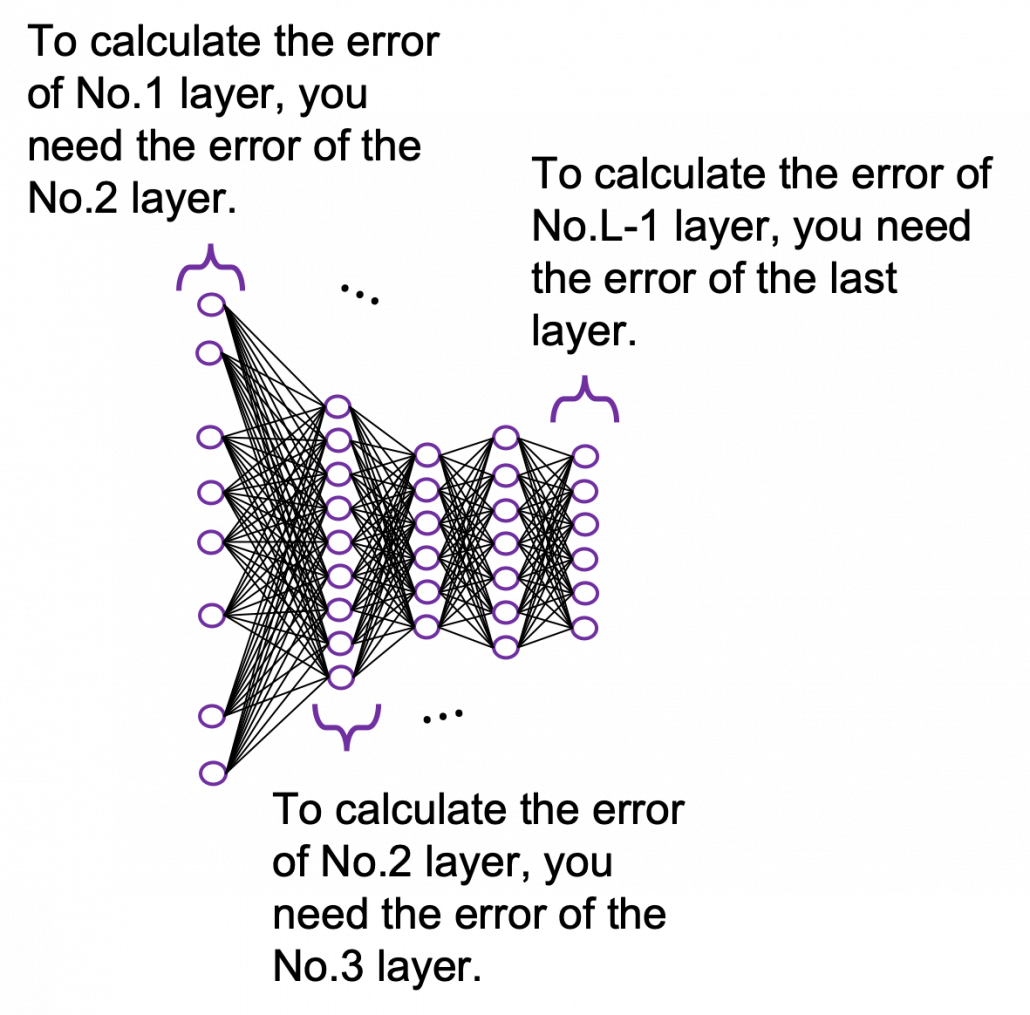
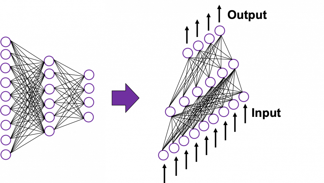In fact the simple RNN which we are going to look at in this article has only three layers. From now on imagine that inputs of RNN come from the bottom and outputs go up. But RNNs have to keep information of earlier times steps during upcoming several time steps because as I mentioned in the last article RNNs are used for sequence data, the order of whose elements is important. In order to do that, information of the neurons in the middle layer of RNN propagate forward to the middle layer itself. Therefore in one time step of forward propagation of RNN, the input at the time step propagates forward as normal DCL, and the RNN gives out an output at the time step. And information of one neuron in the middle layer propagate forward to the other neurons like yellow arrows in the figure. And the information in the next neuron propagate forward to the other neurons, and this process is repeated. This is called recurrent connections of RNN.

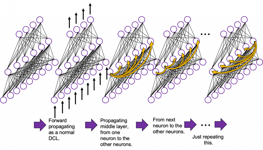
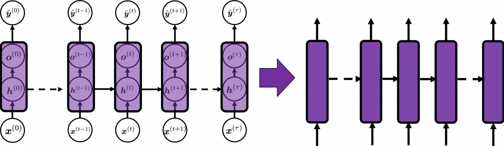
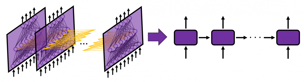
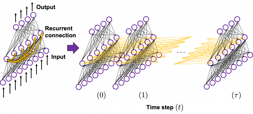*To be exact we are just looking at a type of recurrent connections. For example Elman RNNs have simpler recurrent connections. And recurrent connections of LSTM are more complicated.

Whether it is a simple one or not, basically RNN repeats this process of getting an input at every time step, giving out an output, and making recurrent connections to the RNN itself. But you need to keep the values of activated neurons at every time step, so virtually you need to consider the same RNNs duplicated for several time steps like the figure below. This is the idea of unfolding RNN. Depending on contexts, the whole unfolded DCLs with recurrent connections is also called an RNN.

In many situations, RNNs are simplified as below. If you have read through this article until this point, I bet you gained some better understanding of RNNs, so you should little by little get used to this more abstract, blackboxed way of showing RNN.

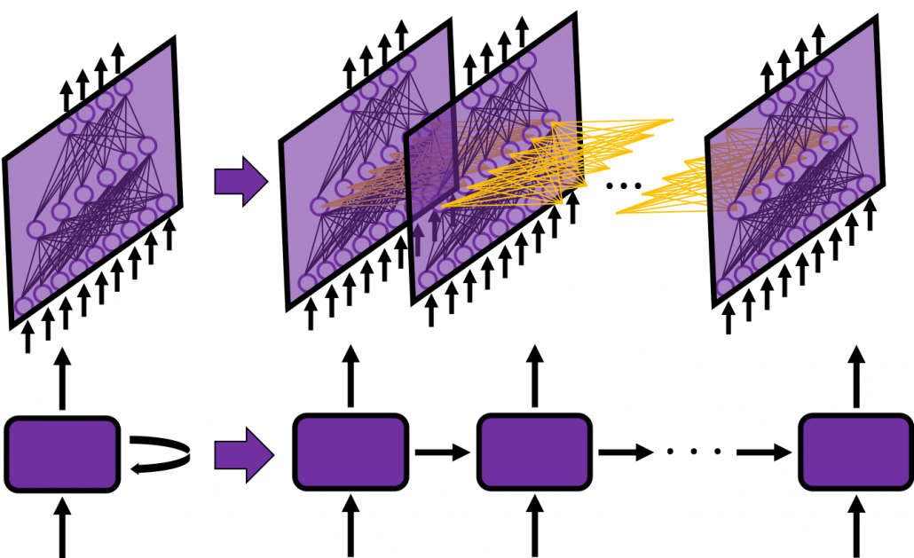
You have seen that you can unfold an RNN, per time step. From now on I am going to show the simple RNN in a simpler way, based on the MIT textbook which I recomment. The figure below shows how RNN propagate forward during two time steps $(t-1), (t)$ .

The input $\boldsymbol{x}^{(t-1)}$ at time step $(t-1)$ propagate forward as a normal DCL, and gives out the output $\hat{\boldsymbol{y}} ^{(t)}$ (The notation on the $\boldsymbol{y} ^{(t)}$ is called “hat,” and it means that the value is an estimated value. Whatever machine learning tasks you work on, the outputs of the functions are just estimations of ideal outcomes. You need to adjust parameters for better estimations. You should always be careful whether it is an actual value or an estimated value in the context of machine learning or statistics). But the most important parts are the middle layers.

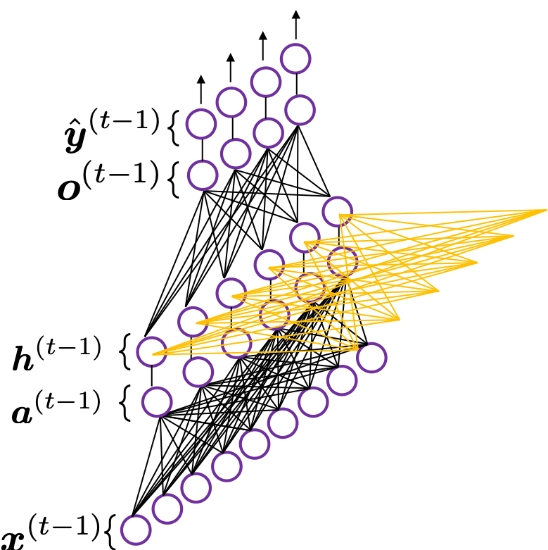
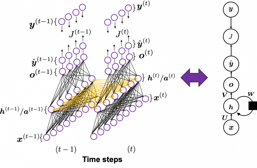
*To be exact I should have drawn the middle layers as connections of two layers of neurons like the figure at the right side. But I made my figure closer to the chart in the MIT textbook, and also most other study materials show the combinations of the two neurons before/after activation as one neuron.

$\boldsymbol{a}^{(t)}$ is just linear summations of $\boldsymbol{x}^{(t)}$ (If you do not know what “linear summations” mean, please scroll this page a bit), and $\boldsymbol{h}^{(t)}$ is a combination of activated values of $\boldsymbol{a}^{(t)}$ and linear summations of $\boldsymbol{h}^{(t-1)}$ from the last time step, with recurrent connections. The values of $\boldsymbol{h}^{(t)}$ propagate forward in two ways. One is normal DCL forward propagation to $\hat{\boldsymbol{y}} ^{(t)}$ and $\boldsymbol{o}^{(t)}$ , and the other is recurrent connections to $\boldsymbol{h}^{(t+1)}$ .

These are equations for each step of forward propagation.

$\boldsymbol{a}^{(t)} = \boldsymbol{b} + \boldsymbol{W} \cdot \boldsymbol{h}^{(t-1)} + \boldsymbol{U} \cdot \boldsymbol{x}^{(t)}$
$\boldsymbol{h}^{(t)}= g(\boldsymbol{a}^{(t)})$
$\boldsymbol{o}^{(t)} = \boldsymbol{c} + \boldsymbol{V} \cdot \boldsymbol{h}^{(t)}$
$\hat{\boldsymbol{y}} ^{(t)} = f(\boldsymbol{o}^{(t)})$

*Please forgive me for adding some mathematical equations on this article even though I pledged not to in the first article. You can skip the them, but for some people it is on the contrary more confusing if there are no equations. In case you are allergic to mathematics, I prescribed some treatments below.

*Linear summation is a type of weighted summation of some elements. Concretely, when you have a vector $\boldsymbol{x}=(x_0, x_1, x_2)$ , and weights $\boldsymbol{w}=(w_0,w_1, w_2)$ , then $\boldsymbol{w}^T \cdot \boldsymbol{x} = w_0 \cdot x_0 + w_1 \cdot x_1 +w_2 \cdot x_2$ is a linear summation of $\boldsymbol{x}$ , and its weights are $\boldsymbol{w}$ .

*When you see a product of a matrix and a vector, for example a product of $\boldsymbol{W}$ and $\boldsymbol{v}$ , you should clearly make an image of connections between two layers of a neural network. You can also say each element of $\boldsymbol{u}}$ is a linear summations all the elements of $\boldsymbol{v}}$ , and $\boldsymbol{W}$ gives the weights for the summations.

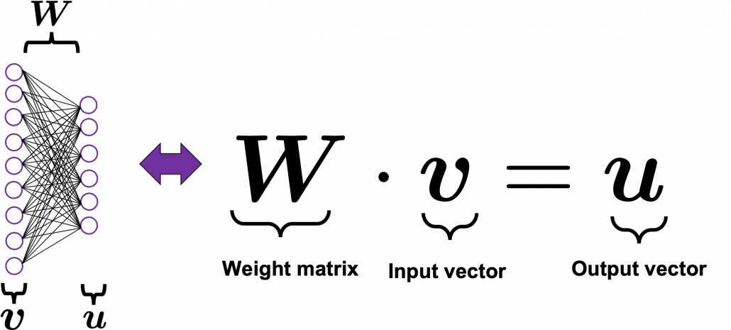
A very important point is that you share the same parameters, in this case $\boldsymbol{\theta \in \{\boldsymbol{U}, \boldsymbol{W}, \boldsymbol{b}, \boldsymbol{V}, \boldsymbol{c} \}}$ , at every time step.

And you are likely to see this RNN in this blackboxed form.

3, The steps of back propagation of simple RNN

In the last article, I said “I have to say backprop of RNN, especially LSTM (a useful and mainstream type or RNN), is a monster of chain rules.” I did my best to make my PowerPoint on LSTM backprop straightforward. But looking at it again, the LSTM backprop part still looks like an electronic circuit, and it requires some patience from you to understand it. If you want to understand LSTM at a more mathematical level, understanding the flow of simple RNN backprop is indispensable, so I would like you to be patient while understanding this step (and you have to be even more patient while understanding LSTM backprop).

This might be a matter of my literacy, but explanations on RNN backprop are very frustrating for me in the points below.

Most explanations just show how to calculate gradients at each time step.
Most study materials are visually very poor.
Most explanations just emphasize that “errors are back propagating through time,” using tons of arrows, but they lack concrete instructions on how actually you renew parameters with those errors.

If you can relate to the feelings I mentioned above, the instructions from now on could somewhat help you. And with the animated PowerPoint slide I prepared, you would have clear understandings on this topic at a more mathematical level.

Backprop of RNN , as long as you are thinking about simple RNNs, is not so different from that of DCLs. But you have to be careful about the meaning of errors in the context of RNN backprop. Back propagation through time (BPTT) is one of the major methods for RNN backprop, and I am sure most textbooks explain BPTT. But most study materials just emphasize that you need errors from all the time steps, and I think that is very misleading and confusing.

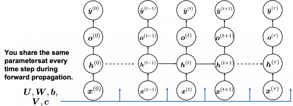
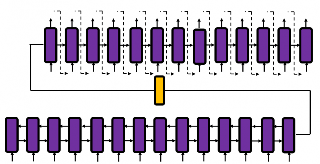
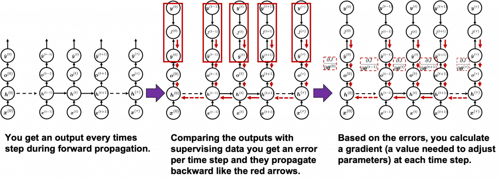You need all the gradients to adjust parameters, but you do not necessarily need all the errors to calculate those gradients. Gradients in the context of machine learning mean partial derivatives of error functions (in this case $J$ ) with respect to certain parameters, and mathematically a gradient of $J$ with respect to $\boldsymbol{\theta \in \{\boldsymbol{U}, \boldsymbol{W}, \boldsymbol{b}^{(t)}, \boldsymbol{V}, \boldsymbol{c} \}}$ is denoted as $( \frac{\partial J}{\partial \boldsymbol{\theta}} )$ . And another confusing point in many textbooks, including the MIT one, is that they give an impression that parameters depend on time steps. For example some study materials use notations like $\frac{\partial J}{\partial \boldsymbol{\theta}^{(t)}}$ , and I think this gives an impression that this is a gradient with respect to the parameters at time step $(t)$ . In my opinion this gradient rather should be written as $( \frac{\partial J}{\partial \boldsymbol{\theta}} )^{(t)}$ . But many study materials denote gradients of those errors in the former way, so from now on let me use the notations which you can see in the figures in this article.

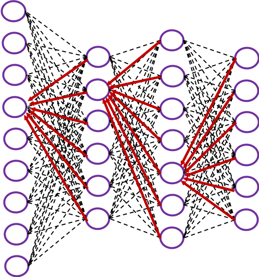
In order to calculate the gradient $\frac{\partial J}{\partial \boldsymbol{x}^{(t)}}$ you need errors from time steps $s (s \geq t) \quad$ (as you can see in the figure, in order to calculate a gradient in a colored frame, you need all the errors in the same color).

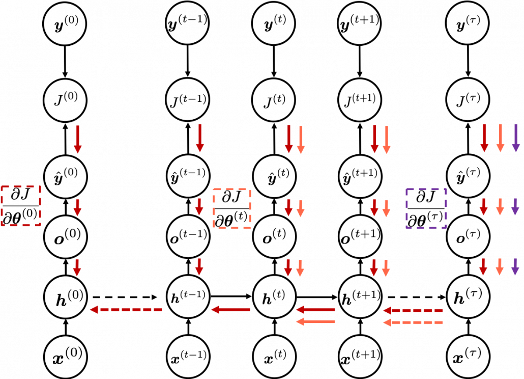
*To be exact, in the figure above I am supposed prepare much more arrows in $\tau + 1$ different colors to show the whole process of RNN backprop, but that is not realistic. In the figure I displayed only the flows of errors necessary for calculating each gradient at time step $0, t, \tau$ .

*Another confusing point is that the $\frac{\partial J}{\partial \boldsymbol{\ast ^{(t)}}}, \boldsymbol{\ast} \in \{\boldsymbol{a}^{(t)}, \boldsymbol{h}^{(t)}, \boldsymbol{o}^{(t)}, \dots \}$ are correct notations, because $\boldsymbol{\ast}$ are values of neurons after forward propagation. They depend on time steps, and these are very values which I have been calling “errors.” That is why parameters do not depend on time steps, whereas errors depend on time steps.

As I mentioned before, you share the same parameters at every time step. Again, please do not assume that parameters are different from time step to time step. It is gradients/errors (you need errors to calculate gradients) which depend on time step. And after calculating errors at every time step, you can finally adjust parameters one time, and that’s why this is called “back propagation through time.” (It is easy to imagine that this method can be very inefficient. If the input is the whole text on a Wikipedia link, you need to input all the sentences in the Wikipedia text to renew parameters one time. To solve this problem there is a backprop method named “truncated BPTT,” with which you renew parameters based on a part of a text. )

And after calculating those gradients $\frac{\partial J}{\partial \boldsymbol{\theta}^{(t)}}$ you can take a summation of them: $\frac{\partial J}{\partial \boldsymbol{\theta}}=\sum_{t=0}^{t=\tau}{\frac{\partial J}{\partial \boldsymbol{\theta}^{(t)}}}$ . With this gradient $\frac{\partial J}{\partial \boldsymbol{\theta}}$ , you can finally renew the value of $\boldsymbol{\theta}$ one time.

At the beginning of this article I mentioned that simple RNNs are no longer for practical uses, and that comes from exploding/vanishing problem of RNN. This problem was one of the reasons for the AI winter which lasted for some 20 years. In the next article I am going to write about LSTM, a fancier type of RNN, in the context of a history of neural network history.

Prerequisites for understanding RNN at a more mathematical level

June 1, 2020/4 Comments/in Artificial Intelligence, Big Data, Data Science, Data Science Hack, Deep Learning, Gerneral, Insights, Machine Learning, Main Category, Natural Language Processing, Text Mining /by Yasuto Tamura

Writing the A gentle introduction to the tiresome part of understanding RNN Article Series on recurrent neural network (RNN) is nothing like a creative or ingenious idea. It is quite an ordinary topic. But still I am going to write my own new article on this ordinary topic because I have been frustrated by lack of sufficient explanations on RNN for slow learners like me.

I think many of readers of articles on this website at least know that RNN is a type of neural network used for AI tasks, such as time series prediction, machine translation, and voice recognition. But if you do not understand how RNNs work, especially during its back propagation, this blog series is for you.

After reading this articles series, I think you will be able to understand RNN in more mathematical and abstract ways. But in case some of the readers are allergic or intolerant to mathematics, I tried to use as little mathematics as possible.

Ideal prerequisite knowledge:

Some understanding on densely connected layers (or fully connected layers, multilayer perception) and how their forward/back propagation work.
Some understanding on structure of Convolutional Neural Network.

*In this article “Densely Connected Layers” is written as “DCL,” and “Convolutional Neural Network” as “CNN.”

1, Difficulty of Understanding RNN

I bet a part of difficulty of understanding RNN comes from the variety of its structures. If you search “recurrent neural network” on Google Image or something, you will see what I mean. But that cannot be helped because RNN enables a variety of tasks.

Another major difficulty of understanding RNN is understanding its back propagation algorithm. I think some of you found it hard to understand chain rules in calculating back propagation of densely connected layers, where you have to make the most of linear algebra. And I have to say backprop of RNN, especially LSTM, is a monster of chain rules. I am planing to upload not only a blog post on RNN backprop, but also a presentation slides with animations to make it more understandable, in some external links.

In order to avoid such confusions, I am going to introduce a very simplified type of RNN, which I call a “simple RNN.” The RNN displayed as the head image of this article is a simple RNN.

2, How Neurons are Connected

How to connect neurons and how to activate them is what neural networks are all about. Structures of those neurons are easy to grasp as long as that is about DCL or CNN. But when it comes to the structure of RNN, many study materials try to avoid showing that RNNs are also connections of neurons, as well as DCL or CNN(*If you are not sure how neurons are connected in CNN, this link should be helpful. Draw a random digit in the square at the corner.). In fact the structure of RNN is also the same, and as long as it is a simple RNN, and it is not hard to visualize its structure.

Even though RNN is also connections of neurons, usually most RNN charts are simplified, using blackboxes. In case of simple RNN, most study material would display it as the chart below.

But that also cannot be helped because fancier RNN have more complicated connections of neurons, and there are no longer advantages of displaying RNN as connections of neurons, and you would need to understand RNN in more abstract way, I mean, as you see in most of textbooks.

I am going to explain details of simple RNN in the next article of this series.

3, Neural Networks as Mappings

If you still think that neural networks are something like magical spider webs or models of brain tissues, forget that. They are just ordinary mappings.

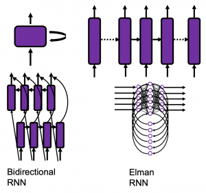
If you have been allergic to mathematics in your life, you might have never heard of the word “mapping.” If so, at least please keep it in mind that the equation $y=f(x)$ , which most people would have seen in compulsory education, is a part of mapping. If you get a value x, you get a value y corresponding to the x.

But in case of deep learning, x is a vector or a tensor, and it is denoted in bold like $\boldsymbol{x}$ . If you have never studied linear algebra , imagine that a vector is a column of Excel data (only one column), a matrix is a sheet of Excel data (with some rows and columns), and a tensor is some sheets of Excel data (each sheet does not necessarily contain only one column.)

CNNs are mainly used for image processing, so their inputs are usually image data. Image data are in many cases (3, hight, width) tensors because usually an image has red, blue, green channels, and the image in each channel can be expressed as a height*width matrix (the “height” and the “width” are number of pixels, so they are discrete numbers).

The convolutional part of CNN (which I call “feature extraction part”) maps the tensors to a vector, and the last part is usually DCL, which works as classifier/regressor. At the end of the feature extraction part, you get a vector. I call it a “semantic vector” because the vector has information of “meaning” of the input image. In this link you can see maps of pictures plotted depending on the semantic vector. You can see that even if the pictures are not necessarily close pixelwise, they are close in terms of the “meanings” of the images.

In the example of a dog/cat classifier introduced by François Chollet, the developer of Keras, the CNN maps (3, 150, 150) tensors to 2-dimensional vectors, (1, 0) or (0, 1) for (dog, cat).

Wrapping up the points above, at least you should keep two points in mind: first, DCL is a classifier or a regressor, and CNN is a feature extractor used for image processing. And another important thing is, feature extraction parts of CNNs map images to vectors which are more related to the “meaning” of the image.

Importantly, I would like you to understand RNN this way. An RNN is also just a mapping.

*I recommend you to at least take a look at the beautiful pictures in this link. These pictures give you some insight into how CNN perceive images.

4, Problems of DCL and CNN, and needs for RNN

Taking an example of RNN task should be helpful for this topic. Probably machine translation is the most famous application of RNN, and it is also a good example of showing why DCL and CNN are not proper for some tasks. Its algorithms is out of the scope of this article series, but it would give you a good insight of some features of RNN. I prepared three sentences in German, English, and Japanese, which have the same meaning. Assume that each sentence is divided into some parts as shown below and that each vector corresponds to each part. In machine translation we want to convert a set of the vectors into another set of vectors.

Then let’s see why DCL and CNN are not proper for such task.

The input size is fixed: In case of the dog/cat classifier I have mentioned, even though the sizes of the input images varies, they were first molded into (3, 150, 150) tensors. But in machine translation, usually the length of the input is supposed to be flexible.
The order of inputs does not mater: In case of the dog/cat classifier the last section, even if the input is “cat,” “cat,” “dog” or “dog,” “cat,” “cat” there’s no difference. And in case of DCL, the network is symmetric, so even if you shuffle inputs, as long as you shuffle all of the input data in the same way, the DCL give out the same outcome . And if you have learned at least one foreign language, it is easy to imagine that the orders of vectors in sequence data matter in machine translation.

*It is said English language has phrase structure grammar, on the other hand Japanese language has dependency grammar. In English, the orders of words are important, but in Japanese as long as the particles and conjugations are correct, the orders of words are very flexible. In my impression, German grammar is between them. As long as you put the verb at the second position and the cases of the words are correct, the orders are also relatively flexible.

5, Sequence Data

We can say DCL and CNN are not useful when you want to process sequence data. Sequence data are a type of data which are lists of vectors. And importantly, the orders of the vectors matter. The number of vectors in sequence data is usually called time steps. A simple example of sequence data is meteorological data measured at a spot every ten minutes, for instance temperature, air pressure, wind velocity, humidity. In this case the data is recorded as 4-dimensional vector every ten minutes.

But this “time step” does not necessarily mean “time.” In case of natural language processing (including machine translation), which you I mentioned in the last section, the numberings of each vector denoting each part of sentences are “time steps.”

And RNNs are mappings from a sequence data to another sequence data.

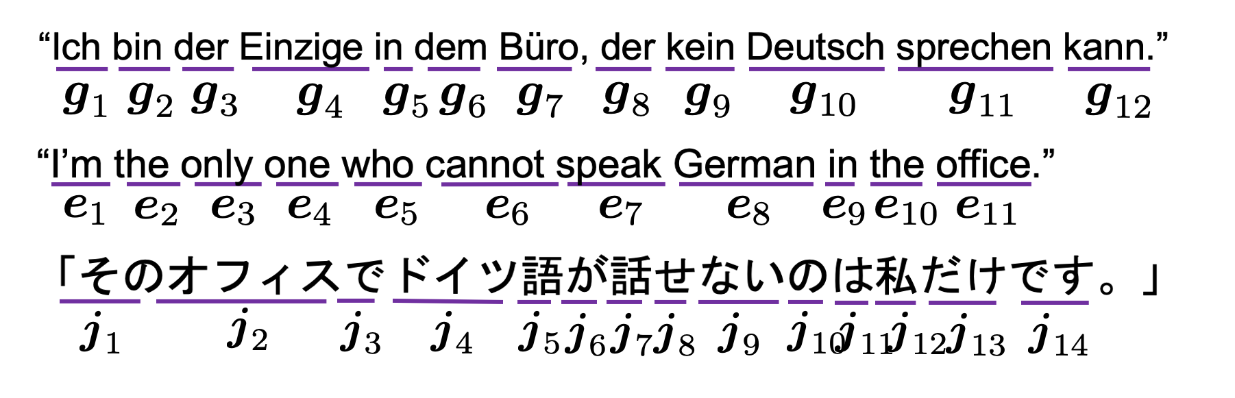
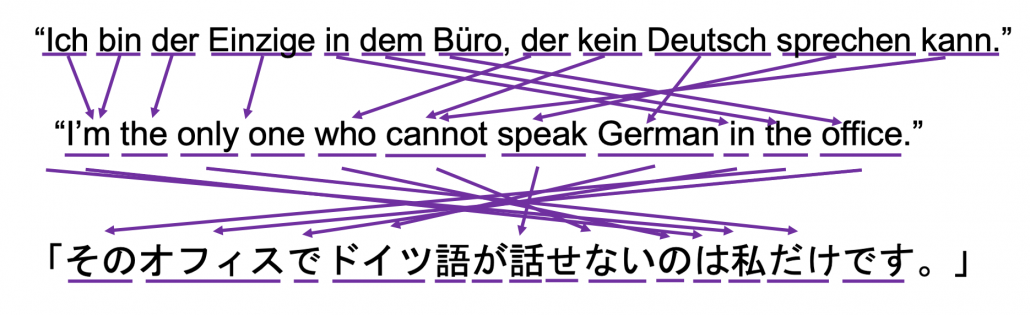
In case of the machine translation above, the each sentence in German, English, and German is expressed as sequence data $\boldsymbol{G}=(\boldsymbol{g}_1,\dots ,\boldsymbol{g}_{12}), \boldsymbol{E}=(\boldsymbol{e}_1,\dots ,\boldsymbol{e}_{11}), \boldsymbol{J}=(\boldsymbol{j}_1,\dots ,\boldsymbol{j}_{14})$ , and machine translation is nothing but mappings between these sequence data.

*At least I found a paper on the RNN’s capability of universal approximation on many-to-one RNN task. But I have not found any papers on universal approximation of many-to-many RNN tasks. Please let me know if you find any clue on whether such approximation is possible. I am desperate to know that.

6, Types of RNN Tasks

RNN tasks can be classified into some types depending on the lengths of input/output sequences (the “length” means the times steps of input/output sequence data).

If you want to predict the temperature in 24 hours, based on several time series data points in the last 96 hours, the task is many-to-one. If you sample data every ten minutes, the input size is 96*6=574 (the input data is a list of 574 vectors), and the output size is 1 (which is a value of temperature). Another example of many-to-one task is sentiment classification. If you want to judge whether a post on SNS is positive or negative, the input size is very flexible (the length of the post varies.) But the output size is one, which is (1, 0) or (0, 1), which denotes (positive, negative).

*The charts in this section are simplified model of RNN used for each task. Please keep it in mind that they are not 100% correct, but I tried to make them as exact as possible compared to those in other study materials.

Music/text generation can be one-to-many tasks. If you give the first sound/word you can generate a phrase.

Next, let’s look at many-to-many tasks. Machine translation and voice recognition are likely to be major examples of many-to-many tasks, but here name entity recognition seems to be a proper choice. Name entity recognition is task of finding proper noun in a sentence . For example if you got two sentences “He said, ‘Teddy bears on sale!’ ” and ‘He said, “Teddy Roosevelt was a great president!” ‘ judging whether the “Teddy” is a proper noun or a normal noun is name entity recognition.

Machine translation and voice recognition, which are more popular, are also many-to-many tasks, but they use more sophisticated models. In case of machine translation, the inputs are sentences in the original language, and the outputs are sentences in another language. When it comes to voice recognition, the input is data of air pressure at several time steps, and the output is the recognized word or sentence. Again, these are out of the scope of this article but I would like to introduce the models briefly.

Machine translation uses a type of RNN named sequence-to-sequence model (which is often called seq2seq model). This model is also very important for other natural language processes tasks in general, such as text summarization. A seq2seq model is divided into the encoder part and the decoder part. The encoder gives out a hidden state vector and it used as the input of the decoder part. And decoder part generates texts, using the output of the last time step as the input of next time step.

Voice recognition is also a famous application of RNN, but it also needs a special type of RNN.

*To be honest, I don’t know what is the state-of-the-art voice recognition algorithm. The example in this article is a combination of RNN and a collapsing function made using Connectionist Temporal Classification (CTC). In this model, the output of RNN is much longer than the recorded words or sentences, so a collapsing function reduces the output into next output with normal length.

You might have noticed that RNNs in the charts above are connected in both directions. Depending on the RNN tasks you need such bidirectional RNNs. I think it is also easy to imagine that such networks are necessary. Again, machine translation is a good example.

And interestingly, image captioning, which enables a computer to describe a picture, is one-to-many-task. As the output is a sentence, it is easy to imagine that the output is “many.” If it is a one-to-many task, the input is supposed to be a vector.

Where does the input come from? I mentioned that the last some layers in of CNN are closely connected to how CNNs extract meanings of pictures. Surprisingly such vectors, which I call a “semantic vectors” is the inputs of image captioning task (after some transformations, depending on the network models).

I think this articles includes major things you need to know as prerequisites when you want to understand RNN at more mathematical level. In the next article, I would like to explain the structure of a simple RNN, and how it forward propagate.

* I make study materials on machine learning, sponsored by DATANOMIQ. I do my best to make my content as straightforward but as precise as possible. I include all of my reference sources. If you notice any mistakes in my materials, please let me know (email: yasuto.tamura@datanomiq.de). And if you have any advice for making my materials more understandable to learners, I would appreciate hearing it.

A gentle introduction to the tiresome part of understanding RNN

May 1, 2020/4 Comments/in Artificial Intelligence, Data Science, Deep Learning, Machine Learning, Mathematics, Uncategorized /by Yasuto Tamura

Just as a normal conversation in a random pub or bar in Berlin, people often ask me “Which language do you use?” I always answer “LaTeX and PowerPoint.”

I have been doing an internship at DATANOMIQ and trying to make straightforward but precise study materials on deep learning. I myself started learning machine learning in April of 2019, and I have been self-studying during this one-year-vacation of mine in Berlin.

Many study materials give good explanations on densely connected layers or convolutional neural networks (CNNs). But when it comes to back propagation of CNN and recurrent neural networks (RNNs), I think there’s much room for improvement to make the topic understandable to learners.

Many study materials avoid the points I want to understand, and that was as frustrating to me as listening to answers to questions in the Japanese Diet, or listening to speeches from the current Japanese minister of the environment. With the slightest common sense, you would always get the feeling “How?” after reading an RNN chapter in any book.

This blog series focuses on the introductory level of recurrent neural networks. By “introductory”, I mean prerequisites for a better and more mathematical understanding of RNN algorithms.

I am going to keep these posts as visual as possible, avoiding equations, but I am also going to attach some links to check more precise mathematical explanations.

This blog series is composed of five contents.:

Prerequisites for understanding RNN at a more mathematical level
Simple RNN: the first foothold for understanding LSTM
A brief history of neural nets: everything you should know before learning LSTM
LSTM and its forward propagation (to be published soon)
LSTM and Its back propagation (to be published soon)

Einführung in die Welt der Autoencoder

April 1, 2020/0 Comments/in Artificial Intelligence, Big Data, Data Mining, Data Science, Data Science Hack, Deep Learning, Main Category, Python, TensorFlow, Tutorial /by Hoang Tu Nguyen

An wen ist der Artikel gerichtet?

In diesem Artikel wollen wir uns näher mit dem neuronalen Netz namens Autoencoder beschäftigen und wollen einen Einblick in die Grundprinzipien bekommen, die wir dann mit einem vereinfachten Programmierbeispiel festigen. Kenntnisse in Python, Tensorflow und neuronalen Netzen sind dabei sehr hilfreich.

Funktionsweise des Autoencoders

Ein Autoencoder ist ein neuronales Netz, welches versucht die Eingangsinformationen zu komprimieren und mit den reduzierten Informationen im Ausgang wieder korrekt nachzubilden.

Die Komprimierung und die Rekonstruktion der Eingangsinformationen laufen im Autoencoder nacheinander ab, weshalb wir das neuronale Netz auch in zwei Abschnitten betrachten können.

Der Encoder

Der Encoder oder auch Kodierer hat die Aufgabe, die Dimensionen der Eingangsinformationen zu reduzieren, man spricht auch von Dimensionsreduktion. Durch diese Reduktion werden die Informationen komprimiert und es werden nur die wichtigsten bzw. der Durchschnitt der Informationen weitergeleitet. Diese Methode hat wie viele andere Arten der Komprimierung auch einen Verlust.

In einem neuronalen Netz wird dies durch versteckte Schichten realisiert. Durch die Reduzierung von Knotenpunkten in den kommenden versteckten Schichten werden die Kodierung bewerkstelligt.

Der Decoder

Nachdem das Eingangssignal kodiert ist, kommt der Decoder bzw. Dekodierer zum Einsatz. Er hat die Aufgabe mit den komprimierten Informationen die ursprünglichen Daten zu rekonstruieren. Durch Fehlerrückführung werden die Gewichte des Netzes angepasst.

Ein bisschen Mathematik

Das Hauptziel des Autoencoders ist, dass das Ausgangssignal dem Eingangssignal gleicht, was bedeutet, dass wir eine Loss Funktion haben, die L(x , y) entspricht.

$L(x, \hat{x})$

Unser Eingang soll mit x gekennzeichnet werden. Unsere versteckte Schicht soll h sein. Damit hat unser Encoder folgenden Zusammenhang h = f(x).

Die Rekonstruktion im Decoder kann mit r = g(h) beschrieben werden. Bei unserem einfachen Autoencoder handelt es sich um ein Feed-Forward Netz ohne rückkoppelten Anteil und wird durch Backpropagation oder zu deutsch Fehlerrückführung optimiert.

Formelzeichen	Bedeutung
$\mathbf{x}, \hat{\mathbf{x}}$	Eingangs-, Ausgangssignal
$\mathbf{W}, \hat{\mathbf{W}}$	Gewichte für En- und Decoder
$\mathbf{B}, \hat{\mathbf{B}}$	Bias für En- und Decoder
$\sigma, \hat{\sigma}$	Aktivierungsfunktion für En- und Decoder
$L$	Verlustfunktion

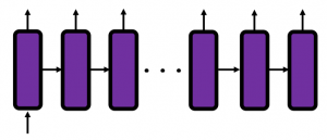
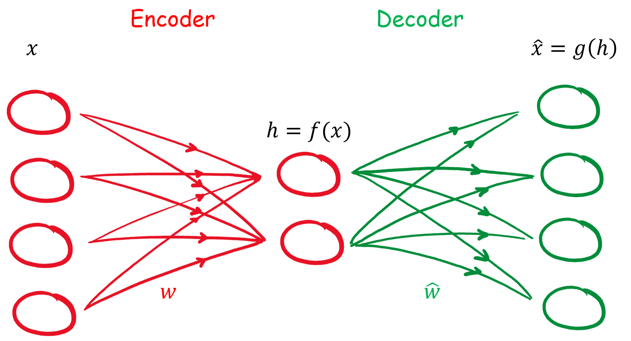
Unsere versteckte Schicht soll mit $\latex h$ gekennzeichnet werden. Damit besteht der Zusammenhang:

(1) $\begin{align*} \mathbf{h} &= f(\mathbf{x}) = \sigma(\mathbf{W}\mathbf{x} + \mathbf{B}) \\ \hat{\mathbf{x}} &= g(\mathbf{h}) = \hat{\sigma}(\hat{\mathbf{W}} \mathbf{h} + \hat{\mathbf{B}}) \\ \hat{\mathbf{x}} &= \hat{\sigma} \{ \hat{\mathbf{W}} \left[\sigma ( \mathbf{W}\mathbf{x} + \mathbf{B} )\right] + \hat{\mathbf{B}} \}\\ \end{align*}$

Für eine Optimierung mit der mittleren quadratischen Abweichung (MSE) könnte die Verlustfunktion wie folgt aussehen:

(2) $\begin{align*} L(\mathbf{x}, \hat{\mathbf{x}}) &= \mathbf{MSE}(\mathbf{x}, \hat{\mathbf{x}}) = \| \mathbf{x} - \hat{\mathbf{x}} \| ^2 &= \| \mathbf{x} - \hat{\sigma} \{ \hat{\mathbf{W}} \left[\sigma ( \mathbf{W}\mathbf{x} + \mathbf{B} )\right] + \hat{\mathbf{B}} \} \| ^2 \end{align*}$

Wir haben die Theorie und Mathematik eines Autoencoder in seiner Ursprungsform kennengelernt und wollen jetzt diese in einem (sehr) einfachen Beispiel anwenden, um zu schauen, ob der Autoencoder so funktioniert wie die Theorie es besagt.

Dazu nehmen wir einen One Hot (1 aus n) kodierten Datensatz, welcher die Zahlen von 0 bis 3 entspricht.

$\begin{align*} [1, 0, 0, 0] \ \widehat{=} \ 0 \\ [0, 1, 0, 0] \ \widehat{=} \ 1 \\ [0, 0, 1, 0] \ \widehat{=} \ 2 \\ [0, 0, 0, 1] \ \widehat{=} \ 3\\ \end{align*}$

Diesen Datensatz könnte wie folgt kodiert werden:

$\begin{align*} [1, 0, 0, 0] \ \widehat{=} \ 0 \ \widehat{=} \ [0, 0] \\ [0, 1, 0, 0] \ \widehat{=} \ 1 \ \widehat{=} \ [0, 1] \\ [0, 0, 1, 0] \ \widehat{=} \ 2 \ \widehat{=} \ [1, 0] \\ [0, 0, 0, 1] \ \widehat{=} \ 3 \ \widehat{=} \ [1, 1] \\ \end{align*}$

Damit hätten wir eine Dimensionsreduktion von vier auf zwei Merkmalen vorgenommen und genau diesen Vorgang wollen wir bei unserem Beispiel erreichen.

Programmierung eines einfachen Autoencoders

Typische Einsatzgebiete des Autoencoders sind neben der Dimensionsreduktion auch Bildaufarbeitung (z.B. Komprimierung, Entrauschen), Anomalie-Erkennung, Sequenz-to-Sequenz Analysen, etc.

Ausblick

Wir haben mit einem einfachen Beispiel die Funktionsweise des Autoencoders festigen können. Im nächsten Schritt wollen wir anhand realer Datensätze tiefer in gehen. Auch soll in kommenden Artikeln Variationen vom Autoencoder in verschiedenen Einsatzgebieten gezeigt werden.

CAPTCHAs lösen via Maschine Learning

March 9, 2020/1 Comment/in Artificial Intelligence, Data Science, Deep Learning, Insights, Machine Learning, Main Category /by Pavel Shipilov

Wie weit ist das maschinelle Lernen auf dem Gebiet der CAPTCHA-Lösung fortgeschritten?

Maschinelles Lernen ist mehr als ein Buzzword, denn unter der Haube stecken viele Algorithemen, die eine ganze Reihe von Problemen lösen können. Die Lösung von CAPTCHA ist dabei nur eine von vielen Aufgaben, die Machine Learning bewältigen kann. Durch die Arbeit an ein paar Problemen im Zusammenhang mit dem konvolutionellen neuronalen Netz haben wir festgestellt, dass es in diesem Bereich noch viel Verbesserungspotenzial gibt. Die Genauigkeit der Erkennung ist oftmals noch nicht gut genug. Schauen wir uns im Einzelnen an, welche Dienste wir haben, um dieses Problem anzugehen, und welche sich dabei als die besten erweisen.

Was ist CAPTCHA?

CAPTCHA ist kein fremder Begriff mehr für Web-Benutzer. Es handelt sich um die ärgerliche menschliche Validierungsprüfung, die auf vielen Websites hinzugefügt wird. Es ist ein Akronym für Completely Automated Public Turing test for tell Computer and Humans Apart. CAPTCHA kann als ein Computerprogramm bezeichnet werden, das dazu entwickelt wurde, Mensch und Maschine zu unterscheiden, um jede Art von illegaler Aktivität auf Websites zu verhindern. Der Sinn von CAPTCHA ist, dass nur ein Mensch diesen Test bestehen können sollte und Bots bzw. irgend eine Form automatisierter Skripte daran versagen. So entsteht ein Wettlauf zwischen CAPTCHA-Anbietern und Hacker-Lösungen, die auf den Einsatz von selbstlernenden Systemen setzen.

Warum müssen wir CAPTCHA lösen?

Heutzutage verwenden die Benutzer automatisierte CAPTCHA-Lösungen für verschiedene Anwendungsfälle. Und hier ein entscheidender Hinweis: Ähnlich wie Penetrationstesting ist der Einsatz gegen Dritte ohne vorherige Genehmigung illegal. Gegen eigene Anwendungen oder gegen Genehmigung (z. B. im Rahmen eines IT-Security-Tests) ist die Anwendung erlaubt. Hacker und Spammer verwenden die CAPTCHA-Bewältigung, um die E-Mail-Adressen der Benutzer zu erhalten, damit sie so viele Spams wie möglich erzeugen können oder um Bruteforce-Attacken durchführen zu können. Die legitimen Beispiele sind Fälle, in denen ein neuer Kunde oder Geschäftspartner zu Ihnen gekommen ist und Zugang zu Ihrer Programmierschnittstelle (API) benötigt, die noch nicht fertig ist oder nicht mit Ihnen geteilt werden kann, wegen eines Sicherheitsproblems oder Missbrauchs, den es verursachen könnte.

Für diese Anwendungsfälle sollen automatisierte Skripte CAPTCHA lösen. Es gibt verschiedene Arten von CAPTCHA: Textbasierte und bildbasierte CAPTCHA, reCAPTCHA und mathematisches CAPTCHA.

Es gibt einen Wettlauf zwischen CAPTCHA-Anbieter und automatisierten Lösungsversuchen. Die in CAPTCHA und reCAPTCHA verwendete Technologie werden deswegen immer intelligenter wird und Aktualisierungen der Zugangsmethoden häufiger. Das Aufrüsten hat begonnen.

Populäre Methoden für die CAPTCHA-Lösung

Die folgenden CAPTCHA-Lösungsmethoden stehen den Benutzern zur Lösung von CAPTCHA und reCAPTCHA zur Verfügung:

OCR (optische Zeichenerkennung) via aktivierte Bots – Dieser spezielle Ansatz löst CAPTCHAs automatisch mit Hilfe der OCR-Technik (Optical Character Recognition). Werkzeuge wie Ocrad, tesseract lösen CAPTCHAs, aber mit sehr geringer Genauigkeit.
Maschinenlernen — Unter Verwendung von Computer Vision, konvolutionalem neuronalem Netzwerk und Python-Frameworks und Bibliotheken wie Keras mit Tensorflow. Wir können tiefe neuronale Konvolutionsnetzmodelle trainieren, um die Buchstaben und Ziffern im CAPTCHA-Bild zu finden.
Online-CAPTCHA-Lösungsdienstleistungen — Diese Dienste verfügen teilweise über menschliche Mitarbeiter, die ständig online verfügbar sind, um CAPTCHAs zu lösen. Wenn Sie Ihre CAPTCHA-Lösungsanfrage senden, übermittelt der Dienst sie an die Lösungsanbieter, die sie lösen und die Lösungen zurückschicken.

Leistungsanalyse der OCR-basierten Lösung

OCR Die OCR ist zwar eine kostengünstige Lösung, wenn es darum geht, eine große Anzahl von trivialen CAPTCHAs zu lösen, aber dennoch liefert sie nicht die erforderliche Genauigkeit. OCR-basierte Lösungen sind nach der Veröffentlichung von ReCaptcha V3 durch Google selten geworden. OCR-fähige Bots sind daher nicht dazu geeignet, CAPTCHA zu umgehen, die von Titanen wie Google, Facebook oder Twitter eingesetzt werden. Hierfür müsste ein besser ausgestattetes CAPTCHA-Lösungssystem eingesetzt werden.

OCR-basierte Lösungen lösen 1 aus 3 trivialen CAPTCHAs korrekt.

Leistungsanalyse der ML-basierten Methode

Schauen wir uns an, wie Lösungen auf dem Prinzip des Maschinenlernens funktionieren:

Die ML-basierte Verfahren verwenden OpenCV, um Konturen in einem Bild zu finden, das die durchgehenden Gebiete feststellt. Die Bilder werden mit der Technik der Schwellenwertbildung vorverarbeitet. Alle Bilder werden in Schwarzweiß konvertiert. Wir teilen das CAPTCHA-Bild mit der OpenCV-Funktion findContour() in verschiedene Buchstaben auf. Die verarbeiteten Bilder sind jetzt nur noch einzelne Buchstaben und Ziffern. Diese werden dann dem CNN-Modell zugeführt, um es zu trainieren. Und das trainierte CNN-Modell ist bereit, die richtige Captchas zu lösen.

Die Präzision einer solchen Lösung ist für alle textbasierten CAPTCHAs weitaus besser als die OCR-Lösung. Es gibt auch viele Nachteile dieser Lösung, denn sie löst nur eine bestimmte Art von CAPTCHAs und Google aktualisiert ständig seinen reCAPTCHA-Generierungsalgorithmus. Die letzte Aktualisierung schien die beste ReCaptcha-Aktualisierung zu sein, die disen Dienst bisher beeinflusst hat: Die regelmäßigen Nutzer hatten dabei kaum eine Veränderung der Schwierigkeit gespürt, während automatisierte Lösungen entweder gar nicht oder nur sehr langsam bzw. inakkurat funktionierten.

Das Modell wurde mit 1⁰⁴ Iterationen mit korrekten und zufälligen Stichproben und 1⁰⁵ Testbildern trainiert, und so wurde eine mittlere Genauigkeit von ~60% erreicht.

Bild-Quelle: “CAPTCHA Recognition with Active Deep Learning” @ TU München https://www.researchgate.net/publication/301620459_CAPTCHA_Recognition_with_Active_Deep_Learning

Wenn Ihr Anwendungsfall also darin besteht, eine Art von CAPTCHA mit ziemlich einfacher Komplexität zu lösen, können Sie ein solches trainiertes ML-Modell hervorragend nutzen. Eine bessere Captcha-Lösungslösung als OCR, muss aber noch eine ganze Menge Bereiche umfassen, um die Genauigkeit der Lösung zu gewährleisten.

Online-Captcha-Lösungsdienst

Online-CAPTCHA-Lösungsdienste sind bisher die bestmögliche Lösung für dieses Problem. Sie verfolgen alle Aktualisierungen von reCAPTCHA durch Google und bieten eine tadellose Genauigkeit von 99%.

Warum sind Online-Anti-Captcha-Dienste leistungsfähiger als andere Methoden?

Die OCR-basierten und ML-Lösungen weisen nach den bisherigen Forschungsarbeiten und Weiterentwicklungen viele Nachteile auf. Sie können nur triviale CAPTCHAs ohne wesentliche Genauigkeit lösen. Hier sind einige Punkte, die in diesem Zusammenhang zu berücksichtigen sind:

– Ein höherer Prozentsatz an korrekten Lösungen (OCR gibt bei wirklich komplizierten CAPTCHAs ein extrem hohes Maß an falschen Antworten; ganz zu schweigen davon, dass einige Arten von CAPTCHA überhaupt nicht mit OCR gelöst werden können, zumindest vorerst).

– Kontinuierlich fehlerfreie Arbeit ohne Unterbrechungen mit schneller Anpassung an die neu hinzugekommene Komplexität.

– Kostengünstig mit begrenzten Ressourcen und geringen Wartungskosten, da es keine Software- oder Hardwareprobleme gibt; alles, was Sie benötigen, ist eine Internetverbindung, um einfache Aufträge über die API des Anti-Captcha-Dienstes zu senden.

Die großen Anbieter von Online-Lösungsdiensten

Jetzt, nachdem wir die bessere Technik zur Lösung Ihrer CAPTCHAs geklärt haben, wollen wir unter allen Anti-Captcha-Diensten den besten auswählen. Einige Dienste bieten eine hohe Genauigkeit der Lösungen, API-Unterstützung für die Automatisierung und schnelle Antworten auf unsere Anfragen. Dazu gehören Dienste wie 2captcha, Imagetyperz, CaptchaSniper, etc.

2CAPTCHA ist einer der Dienste, die auf die Kombination von Machine Learning und echten Menschen setzen, um CAPTCHA zuverlässig zu lösen. Dabei versprechen Dienste wie 2captcha:

Schnelle Lösung mit 17 Sekunden für grafische und textuelle Captchas und ~23 Sekunden für ReCaptcha
Unterstützt alle populären Programmiersprachen mit einer umfassenden Dokumentation der fertigen Bibliotheken.
Hohe Genauigkeit (bis zu 99% je nach dem CAPTCHA-Typ).
Das Geld wird bei falschen Antworten zurückerstattet.
Fähigkeit, eine große Anzahl von Captchas zu lösen (mehr als 10.000 pro Minute)

Schlussfolgerung

Convolutional Neural Networks (CNN) wissen, wie die einfachsten Arten von Captcha zu bewältigen sind und werden auch mit der weiteren Enwicklung schritthalten können. Wir haben es mit einem Wettlauf um verkomplizierte CAPTCHAs und immer fähigeren Lösungen der automatisierten Erkennung zutun. Zur Zeit werden Online-Anti-Captcha-Dienste, die auf einen Mix aus maschinellem Lernen und menschlicher Intelligenz setzen, diesen Lösungen vorerst voraus sein.

Visual Question Answering with Keras – Part 1

July 29, 2019/0 Comments/in Artificial Intelligence, Data Science, Data Science Hack, Deep Learning, Insights, Machine Learning, Main Category, Predictive Analytics, TensorFlow /by Akshay Chavan

This is Part I of II of the Article Series Visual Question Answering with Keras

Making Computers Intelligent to answer from images

If we look closer in the history of Artificial Intelligence (AI), the Deep Learning has gained more popularity in the recent years and has achieved the human-level performance in the tasks such as Speech Recognition, Image Classification, Object Detection, Machine Translation and so on. However, as humans, not only we but also a five-year child can normally perform these tasks without much inconvenience. But the development of such systems with these capabilities has always considered an ambitious goal for the researchers as well as for developers.

In this series of blog posts, I will cover an introduction to something called VQA (Visual Question Answering), its available datasets, the Neural Network approach for VQA and its implementation in Keras and the applications of this challenging problem in real life.

Table of Contents:

1 Introduction

2 What is exactly Visual Question Answering?

3 Prerequisites

4 Datasets available for VQA

4.1 DAQUAR Dataset

4.2 CLEVR Dataset

4.3 FigureQA Dataset

4.4 VQA Dataset

5 Real-life applications of VQA

6 Conclusion

Introduction:

Let’s say you are given a below picture along with one question. Can you answer it?

I expect confidently you all say it is the Kitchen without much inconvenience which is also the right answer. Even a five-year child who just started to learn things might answer this question correctly.

Alright, but can you write a computer program for such type of task that takes image and question about the image as an input and gives us answer as output?

Before the development of the Deep Neural Network, this problem was considered as one of the difficult, inconceivable and challenging problem for the AI researcher’s community. However, due to the recent advancement of Deep Learning the systems are capable of answering these questions with the promising result if we have a required dataset.

Now I hope you have got at least some intuition of a problem that we are going to discuss in this series of blog posts. Let’s try to formalize the problem in the below section.

What is exactly Visual Question Answering?:

We can define, “Visual Question Answering(VQA) is a system that takes an image and natural language question about the image as an input and generates natural language answer as an output.”

VQA is a research area that requires an understanding of vision(Computer Vision) as well as text(NLP). The main beauty of VQA is that the reasoning part is performed in the context of the image. So if we have an image with the corresponding question then the system must able to understand the image well in order to generate an appropriate answer. For example, if the question is the number of persons then the system must able to detect faces of the persons. To answer the color of the horse the system need to detect the objects in the image. Many of these common problems such as face detection, object detection, binary object classification(yes or no), etc. have been solved in the field of Computer Vision with good results.

To summarize a good VQA system must be able to address the typical problems of CV as well as NLP.

To get a better feel of VQA you can try online VQA demo by CloudCV. You just go to this link and try uploading the picture you want and ask the related question to the picture, the system will generate the answer to it.

Prerequisites:

In the next post, I will walk you through the code for this problem using Keras. So I assume that you are familiar with:

Fundamental concepts of Machine Learning
Multi-Layered Perceptron
Convolutional Neural Network
Recurrent Neural Network (especially LSTM)
Gradient Descent and Backpropagation
Transfer Learning
Hyperparameter Optimization
Python and Keras syntax

Datasets available for VQA:

As you know problems related to the CV or NLP the availability of the dataset is the key to solve the problem. The complex problems like VQA, the dataset must cover all possibilities of questions answers in real-world scenarios. In this section, I will cover some of the datasets available for VQA.

4.1 DAQUAR Dataset:

The DAQUAR dataset is the first dataset for VQA that contains only indoor scenes. It shows the accuracy of 50.2% on the human baseline. It contains images from the NYU_Depth dataset.

Example of DAQUAR dataset

The main disadvantage of DAQUAR is the size of the dataset is very small to capture all possible indoor scenes.

4.2 CLEVR Dataset:

The CLEVR Dataset from Stanford contains the questions about the object of a different type, colors, shapes, sizes, and material.

It has

A training set of 70,000 images and 699,989 questions
A validation set of 15,000 images and 149,991 questions
A test set of 15,000 images and 14,988 questions

Image Source: https://cs.stanford.edu/people/jcjohns/clevr/?source=post_page

4.3 FigureQA Dataset:

FigureQA Dataset contains questions about the bar graphs, line plots, and pie charts. It has 1,327,368 questions for 100,000 images in the training set.

4.4 VQA Dataset:

As comapred to all datasets that we have seen so far VQA dataset is relatively larger. The VQA dataset contains open ended as well as multiple choice questions. VQA v2 dataset contains:

82,783 training images from COCO (common objects in context) dataset
40, 504 validation images and 81,434 validation images
443,757 question-answer pairs for training images
214,354 question-answer pairs for validation images.

As you might expect this dataset is very huge and contains 12.6 GB of training images only. I have used this dataset in the next post but a very small subset of it.

This dataset also contains abstract cartoon images. Each image has 3 questions and each question has 10 multiple choice answers.

Real-life applications of VQA:

There are many applications of VQA. One of the famous applications is to help visually impaired people and blind peoples. In 2016, Microsoft has released the “Seeing AI” app for visually impaired people to describe the surrounding environment around them. You can watch this video for the prototype of the Seeing AI app.

Another application could be on social media or e-commerce sites. VQA can be also used for educational purposes.

Conclusion:

I hope this explanation will give you a good idea of Visual Question Answering. In the next blog post, I will walk you through the code in Keras.

If you like my explanations, do provide some feedback, comments, etc. and stay tuned for the next post.

Introduction to ROC Curve

April 9, 2019/0 Comments/in Artificial Intelligence, Data Mining, Data Science, Deep Learning, Machine Learning, Main Category, Predictive Analytics /by rohitmishra

The abbreviation ROC stands for Receiver Operating Characteristic. Its main purpose is to illustrate the diagnostic ability of classifier as the discrimination threshold is varied. It was developed during World War II when Radar operators had to decide if the blip on the screen is an enemy target, a friendly ship or just a noise. For these purposes they measured the ability of a radar receiver operator to make these important distinctions, which was called the Receiver Operating Characteristic.

Later it was found useful in interpreting medical test results and then in Machine learning classification problems. In order to get an introduction to binary classification and terms like ‘precision’ and ‘recall’ one can look into my earlier blog here.

True positive rate and false positive rate

Let’s imagine a situation where a fire alarm is installed in a kitchen. The alarm is supposed to emit a sound in case fire smoke is detected in the room. Unfortunately, there is a lot of cooking done in the kitchen and the alarm may trigger the sound too often. Thus, instead of serving a purpose the alarm becomes a nuisance due to a large number of false alarms. In statistical terms these types of errors are called type 1 errors, or false positives.

One way to deal with this problem is to simply decrease sensitivity of the device. We do this by increasing the trigger threshold at the alarm setting. But then, not every alarm should have the same threshold setting. Consider the same type of device but kept in a bedroom. With high threshold, the device might miss smoke from a real short-circuit in the wires which poses a real danger of fire. This kind of failure is called Type 2 error or a false negative. Although the two devices are the same, different types of threshold settings are optimal for different circumstances.

To specify this more formally, let us describe the performance of a binary classifier at a particular threshold by the following parameters:

These parameters take different values at different thresholds. Hence, they define the performance of the classifier at particular threshold. But we want to examine in overall how good a classifier is. Fortunately, there is a way to do that. We plot the True Positive Rate (TPR) and False Positive rate (FPR) at different thresholds and this plot is called ROC curve.

Let’s try to understand this with an example.

A case with a distinct population distribution

Let’s suppose there is a disease which can be identified with deficiency of some parameter (maybe a certain vitamin). The distribution of population with this disease has a mean vitamin concentration sharply distinct from the mean of a healthy population, as shown below.

This is result of dummy data simulating population of 2000 people,the link to the code is given in the end of this blog. As the two populations are distinctly separated (there is no overlap between the two distributions), we can expect that a classifier would have an easy job distinquishing healthy from sick people. We can run a logistic regression classifier with a threshold of .5 and be 100% succesful in detecting the decease.

The confusion matrix may look something like this.

In this ideal case with a threshold of .5 we do not make a single wrong classification. The True positive rate and False positive rate are 1 and 0, respectively. But we can shift the threshold. In that case, we will get different confusion matrices. First we plot threshold vs. TPR.

We see for most values of threshold the TPR is close to 1 which again proves data is easy to classify and the classifier is returning high probabilities for the most of positives .

Similarly Let’s plot threshold vs. FPR.

For most of the data points FPR is close to zero. This is also good. Now its time to plot the ROC curve using these results (TPR vs FPR).

Let’s try to interpret the results, all the points lie on line x=0 and y=1, it means for all the points FPR is zero or TPR is one, making the curve a square. which means the classifier does perfectly well.

Case with overlapping population distribution

The above example was about a perfect classifer. However, life is often not so easy. Now let us consider another more realistic situation in which the parameter distribution of the population is not as distinct as in the previous case. Rather, the mean of the parameter with healthy and not healthy datapoints are close and the distributions overlap, as shown in the next figure.

If we set the threshold to 0.5, the confusion matrix may look like this.

Now, any new choice of threshold location will affect both false positives and false negatives. In fact, there is a trade-off. If we shift the threshold with the goal to reduce false negatives, false positives will increase. If we move the threshold to the other direction and reduce false positive, false negatives will increase.

The plots (TPR vs Threshold) , (FPR vs Threshold) are shown below

If we plot the ROC curve from these results, it looks like this:

From the curve we see the classifier does not perform as well as the earlier one.

What else can be infered from this curve? We first need to understand what the diagonal in this plot represent. The diagonal represents ‘Line of no discrimination’, which we obtain if we randomly guess. This is the ROC curve for the worst possible classifier. Therefore, by comparing the obtained ROC curve with the diagonal, we see how much better our classifer is from random guessing.

The further away ROC curve from the diagonal is (the closest it is to the top left corner) , better the classifier is.

Area Under the curve

The overall performance of the classifier is given by the area under the ROC curve and is usually denoted as AUC. Since TPR and FPR lie within the range of 0 to 1, the AUC also assumes values between 0 and 1. The higher the value of AUC, the better is the overall performance of the classifier.

Let’s see this for the two different distributions which we saw earlier.

As we know the classifier had worked perfectly in the first case with points at (0,1) the area under the curve is 1 which is perfect. In the latter case the classifier was not able to perform as good, the ROC curve is between the diagonal and left hand corner. The AUC as we can see is less than 1.

Some other general characteristics

There are still few points that needs to be discussed on a General ROC curve

The ROC curve does not provide information about the actual values of thresholds used for the classifier.
Performance of different classifiers can be compared using the AUC of different Classifier. The larger the AUC, the better the classifier.
The vertical distance of the ROC curve from the no discrimination line gives a measure of ‘INFORMEDNESS’. This is known as Youden’s J satistic. This statistics can take values between 0 and 1.

Youden’s J statistic is defined for every point on the ROC curve . The point at which Youden’s J satistics reaches its maximum for a given ROC curve can be used to guide the selection of the threshold to be used for that classifier.

I hope this post does the job of providing an understanding of ROC curves and AUC. The Python program for simulating the example given earlier can be found here .

Please feel free to adjust the mean of the distributions and see the changes in the plot.

1. Preface

2. Why LSTM?

3. How to display LSTM

4. Forward propagation of LSTM in “electronic circuit type”

5. Space Odyssey type

1, First AI boom

2, Second AI boom/winter

3, Video game industry and GPU

4, Pretraining of deep belief networks: “The Dawn of Deep Learning”

1, A brief review on back propagation of DCL.

2, Forward propagation of simple RNN

3, The steps of back propagation of simple RNN

1, Difficulty of Understanding RNN

2, How Neurons are Connected

3, Neural Networks as Mappings

4, Problems of DCL and CNN, and needs for RNN

5, Sequence Data

6, Types of RNN Tasks

This blog series is composed of five contents.:

An wen ist der Artikel gerichtet?

Funktionsweise des Autoencoders

Der Encoder

Der Decoder

Ein bisschen Mathematik

Programmierung eines einfachen Autoencoders

Ausblick

Wie weit ist das maschinelle Lernen auf dem Gebiet der CAPTCHA-Lösung fortgeschritten?

Was ist CAPTCHA?

Warum müssen wir CAPTCHA lösen?

Populäre Methoden für die CAPTCHA-Lösung

Leistungsanalyse der OCR-basierten Lösung

Leistungsanalyse der ML-basierten Methode

Online-Captcha-Lösungsdienst

Die großen Anbieter von Online-Lösungsdiensten

Schlussfolgerung

True positive rate and false positive rate

A case with a distinct population distribution

Case with overlapping population distribution

Area Under the curve

Some other general characteristics

Interesting links

Pages

Categories

Archive