
Introduction to ROC Curve
The abbreviation ROC stands for Receiver Operating Characteristic. Its main purpose is to illustrate the diagnostic ability of classifier as the discrimination threshold is varied. It was developed during World War II when Radar operators had to decide if the blip on the screen is an enemy target, a friendly ship or just a noise. For these purposes they measured the ability of a radar receiver operator to make these important distinctions, which was called the Receiver Operating Characteristic.
Later it was found useful in interpreting medical test results and then in Machine learning classification problems. In order to get an introduction to binary classification and terms like ‘precision’ and ‘recall’ one can look into my earlier blog here.
True positive rate and false positive rate
Let’s imagine a situation where a fire alarm is installed in a kitchen. The alarm is supposed to emit a sound in case fire smoke is detected in the room. Unfortunately, there is a lot of cooking done in the kitchen and the alarm may trigger the sound too often. Thus, instead of serving a purpose the alarm becomes a nuisance due to a large number of false alarms. In statistical terms these types of errors are called type 1 errors, or false positives.
One way to deal with this problem is to simply decrease sensitivity of the device. We do this by increasing the trigger threshold at the alarm setting. But then, not every alarm should have the same threshold setting. Consider the same type of device but kept in a bedroom. With high threshold, the device might miss smoke from a real short-circuit in the wires which poses a real danger of fire. This kind of failure is called Type 2 error or a false negative. Although the two devices are the same, different types of threshold settings are optimal for different circumstances.
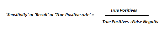
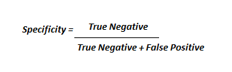
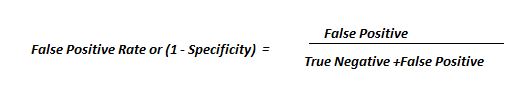
To specify this more formally, let us describe the performance of a binary classifier at a particular threshold by the following parameters:
These parameters take different values at different thresholds. Hence, they define the performance of the classifier at particular threshold. But we want to examine in overall how good a classifier is. Fortunately, there is a way to do that. We plot the True Positive Rate (TPR) and False Positive rate (FPR) at different thresholds and this plot is called ROC curve.
Let’s try to understand this with an example.
A case with a distinct population distribution
Let’s suppose there is a disease which can be identified with deficiency of some parameter (maybe a certain vitamin). The distribution of population with this disease has a mean vitamin concentration sharply distinct from the mean of a healthy population, as shown below.
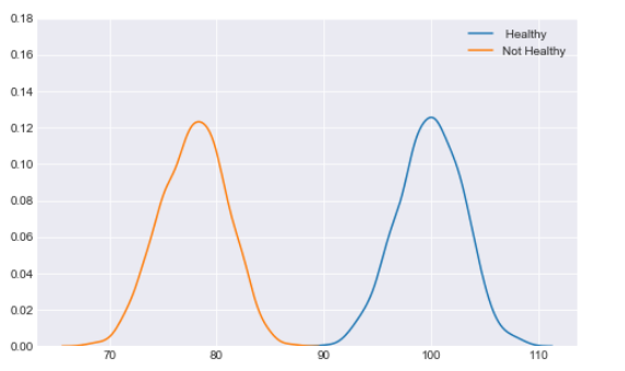
This is result of dummy data simulating population of 2000 people,the link to the code is given in the end of this blog. As the two populations are distinctly separated (there is no overlap between the two distributions), we can expect that a classifier would have an easy job distinquishing healthy from sick people. We can run a logistic regression classifier with a threshold of .5 and be 100% succesful in detecting the decease.
The confusion matrix may look something like this.
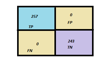
In this ideal case with a threshold of .5 we do not make a single wrong classification. The True positive rate and False positive rate are 1 and 0, respectively. But we can shift the threshold. In that case, we will get different confusion matrices. First we plot threshold vs. TPR.
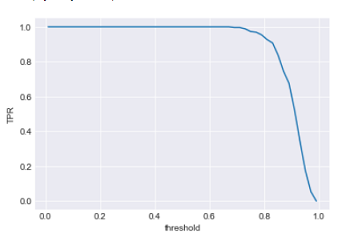
We see for most values of threshold the TPR is close to 1 which again proves data is easy to classify and the classifier is returning high probabilities for the most of positives .
Similarly Let’s plot threshold vs. FPR.
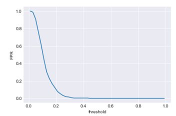
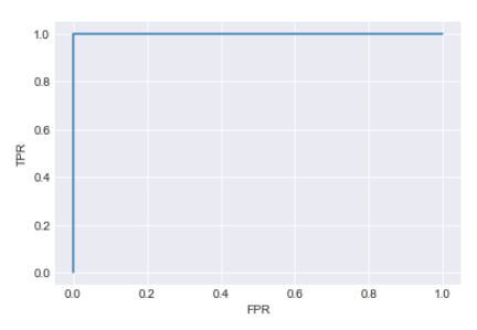
For most of the data points FPR is close to zero. This is also good. Now its time to plot the ROC curve using these results (TPR vs FPR).
Let’s try to interpret the results, all the points lie on line x=0 and y=1, it means for all the points FPR is zero or TPR is one, making the curve a square. which means the classifier does perfectly well.
Case with overlapping population distribution
The above example was about a perfect classifer. However, life is often not so easy. Now let us consider another more realistic situation in which the parameter distribution of the population is not as distinct as in the previous case. Rather, the mean of the parameter with healthy and not healthy datapoints are close and the distributions overlap, as shown in the next figure.
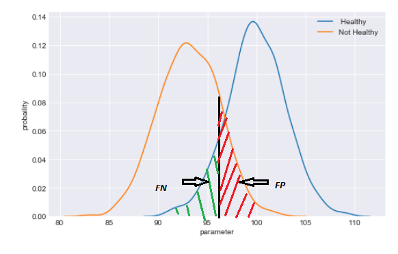
If we set the threshold to 0.5, the confusion matrix may look like this.
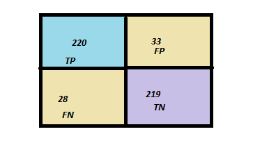
Now, any new choice of threshold location will affect both false positives and false negatives. In fact, there is a trade-off. If we shift the threshold with the goal to reduce false negatives, false positives will increase. If we move the threshold to the other direction and reduce false positive, false negatives will increase.
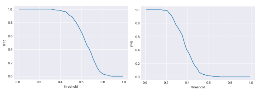
The plots (TPR vs Threshold) , (FPR vs Threshold) are shown below
If we plot the ROC curve from these results, it looks like this:
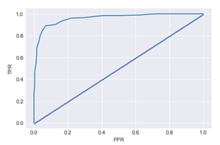
From the curve we see the classifier does not perform as well as the earlier one.
What else can be infered from this curve? We first need to understand what the diagonal in this plot represent. The diagonal represents ‘Line of no discrimination’, which we obtain if we randomly guess. This is the ROC curve for the worst possible classifier. Therefore, by comparing the obtained ROC curve with the diagonal, we see how much better our classifer is from random guessing.
The further away ROC curve from the diagonal is (the closest it is to the top left corner) , better the classifier is.
Area Under the curve
The overall performance of the classifier is given by the area under the ROC curve and is usually denoted as AUC. Since TPR and FPR lie within the range of 0 to 1, the AUC also assumes values between 0 and 1. The higher the value of AUC, the better is the overall performance of the classifier.
Let’s see this for the two different distributions which we saw earlier.
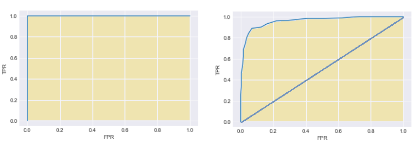
As we know the classifier had worked perfectly in the first case with points at (0,1) the area under the curve is 1 which is perfect. In the latter case the classifier was not able to perform as good, the ROC curve is between the diagonal and left hand corner. The AUC as we can see is less than 1.
Some other general characteristics
There are still few points that needs to be discussed on a General ROC curve
- The ROC curve does not provide information about the actual values of thresholds used for the classifier.
- Performance of different classifiers can be compared using the AUC of different Classifier. The larger the AUC, the better the classifier.
- The vertical distance of the ROC curve from the no discrimination line gives a measure of ‘INFORMEDNESS’. This is known as Youden’s J satistic. This statistics can take values between 0 and 1.
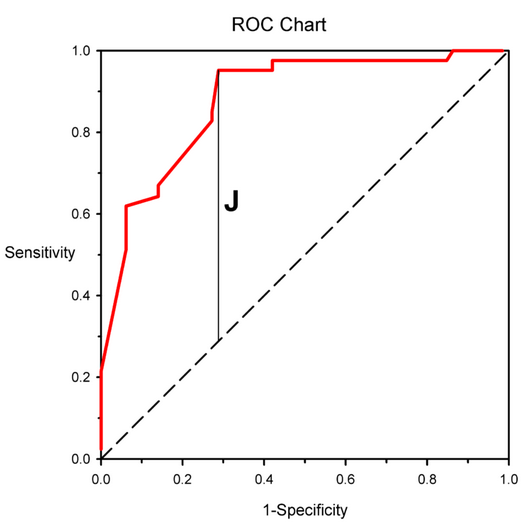
Youden’s J statistic is defined for every point on the ROC curve . The point at which Youden’s J satistics reaches its maximum for a given ROC curve can be used to guide the selection of the threshold to be used for that classifier.
I hope this post does the job of providing an understanding of ROC curves and AUC. The Python program for simulating the example given earlier can be found here .
Please feel free to adjust the mean of the distributions and see the changes in the plot.
rohitmishra
Rohit has worked as screenwriter for films and Science Documentaries in Mumbai. Having a strong passion towards Math and science, he got drawn towards data Science and artificial intelligence. His love for science and storytelling drives him to write scientific blogs. Currently Rohit works as an intern in Data Science team in Savedroid AG in Frankfurt.


Leave a Reply
Want to join the discussion?Feel free to contribute!