Visual Question Answering with Keras – Part 2: Making Computers Intelligent to answer from images

Making Computers Intelligent to answer from images

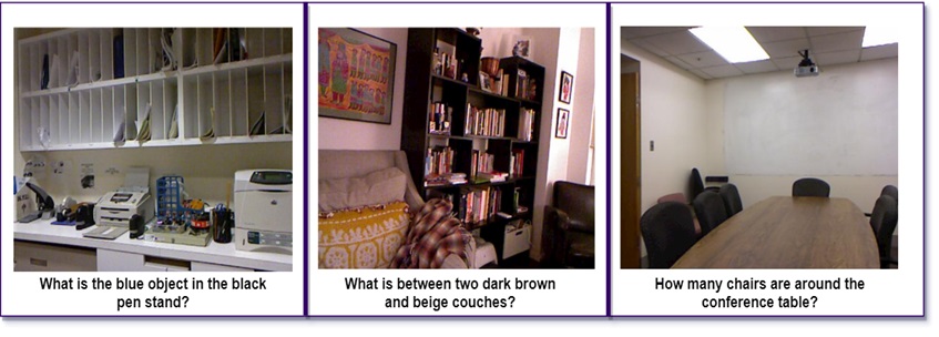
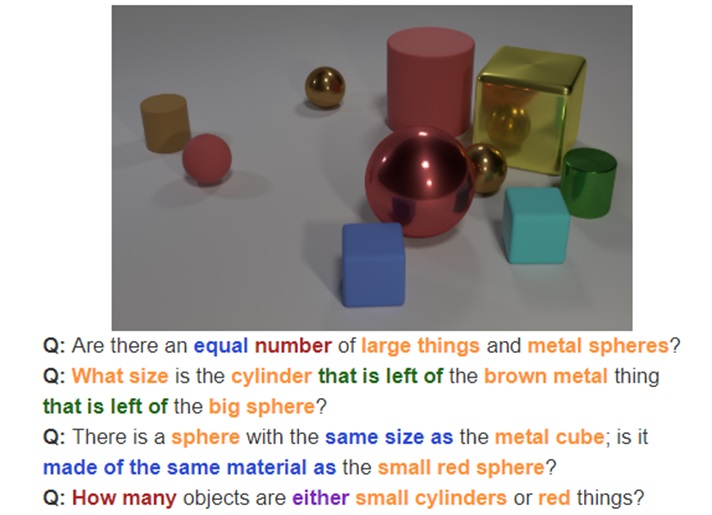
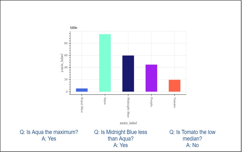
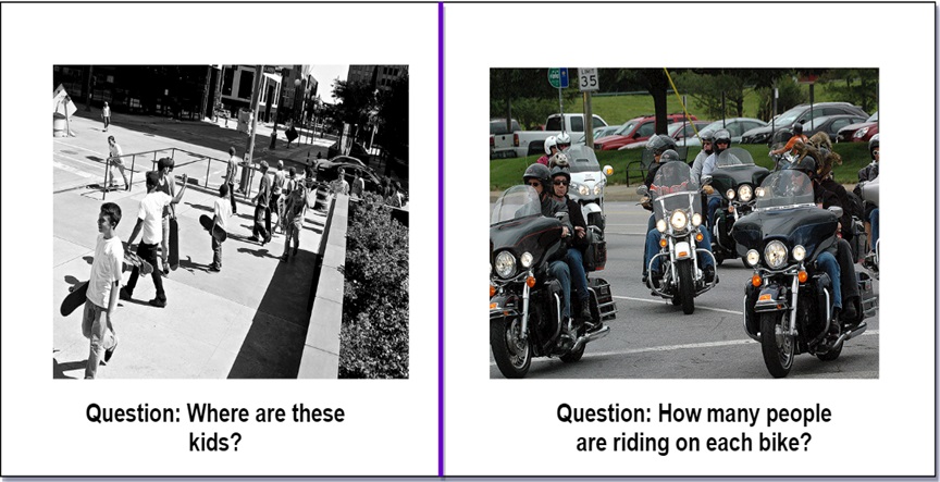
This is my second blog on Visual Question Answering, in the last blog, I have introduced to VQA, available datasets and some of the real-life applications of VQA. If you have not gone through then I would highly recommend you to go through it. Click here for more details about it.

In this blog post, I will walk through the implementation of VQA in Keras.

You can download the dataset from here: https://visualqa.org/index.html. All my experiments were performed with VQA v2 and I have used a very tiny subset of entire dataset i.e all samples for training and testing from the validation set.

Table of contents:

  1. Preprocessing Data
  2. Process overview for VQA
  3. Data Preprocessing – Images
  4. Data Preprocessing through the spaCy library- Questions
  5. Model Architecture
  6. Defining model parameters
  7. Evaluating the model
  8. Final Thought
  9. References

NOTE: The purpose of this blog is not to get the state-of-art performance on VQA. But the idea is to get familiar with the concept. All my experiments were performed with the validation set only.

Full code on my Github here.


1. Preprocessing Data:

If you have downloaded the dataset then the question and answers (called as annotations) are in JSON format. I have provided the code to extract the questions, annotations and other useful information in my Github repository. All extracted information is stored in .txt file format. After executing code the preprocessing directory will have the following structure.

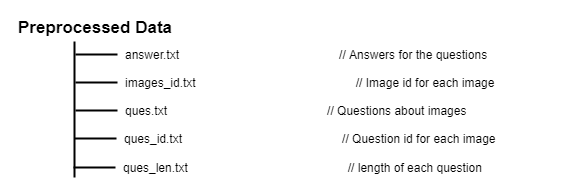
All text files will be used for training.


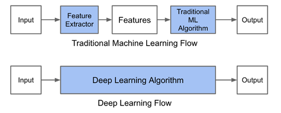
2. Process overview for VQA:

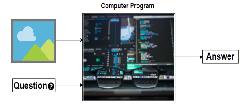
As we have discussed in previous post visual question answering is broken down into 2 broad-spectrum i.e. vision and text.  I will represent the Neural Network approach to this problem using the Convolutional Neural Network (for image data) and Recurrent Neural Network(for text data). 

If you are not familiar with RNN (more precisely LSTM) then I would highly recommend you to go through Colah’s blog and Andrej Karpathy blog. The concepts discussed in this blogs are extensively used in my post.

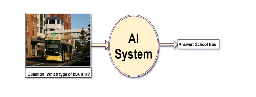
The main idea is to get features for images from CNN and features for the text from RNN and finally combine them to generate the answer by passing them through some fully connected layers. The below figure shows the same idea.
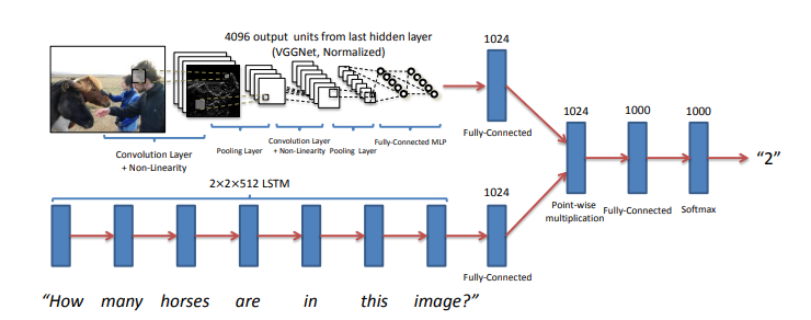
 

I have used VGG-16 to extract the features from the image and LSTM layers to extract the features from questions and combining them to get the answer.

3. Data Preprocessing – Images:

Images are nothing but one of the input to our model. But as you already may know that before feeding images to the model we need to convert into the fixed-size vector.

So we need to convert every image into a fixed-size vector then it can be fed to the neural network. For this, we will use the VGG-16 pretrained model. VGG-16 model architecture is trained on millions on the Imagenet dataset to classify the image into one of 1000 classes. Here our task is not to classify the image but to get the bottleneck features from the second last layer.

Hence after removing the softmax layer, we get a 4096-dimensional vector representation (bottleneck features) for each image.

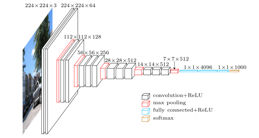
Image Source: https://www.cs.toronto.edu/~frossard/post/vgg16/


For the VQA dataset, the images are from the COCO dataset and each image has unique id associated with it. All these images are passed through the VGG-16 architecture and their vector representation is stored in the “.mat” file along with id. So in actual, we need not have to implement VGG-16 architecture instead we just do look up into file with the id of the image at hand and we will get a 4096-dimensional vector representation for the image.

4. Data Preprocessing through the spaCy library- Questions:

spaCy is a free, open-source library for advanced Natural Language Processing (NLP) in Python. As we have converted images into a fixed 4096-dimensional vector we also need to convert questions into a fixed-size vector representation. For installing spaCy click here

You might know that for training word embeddings in Keras we have a layer called an Embedding layer which takes a word and embeds it into a higher dimensional vector representation. But by using the spaCy library we do not have to train the get the vector representation in higher dimensions.


This model is actually trained on billions of tokens of the large corpus. So we just need to call the vector method of spaCy class and will get vector representation for word.

After fitting, the vector method on tokens of each question will get the 300-dimensional fixed representation for each word.

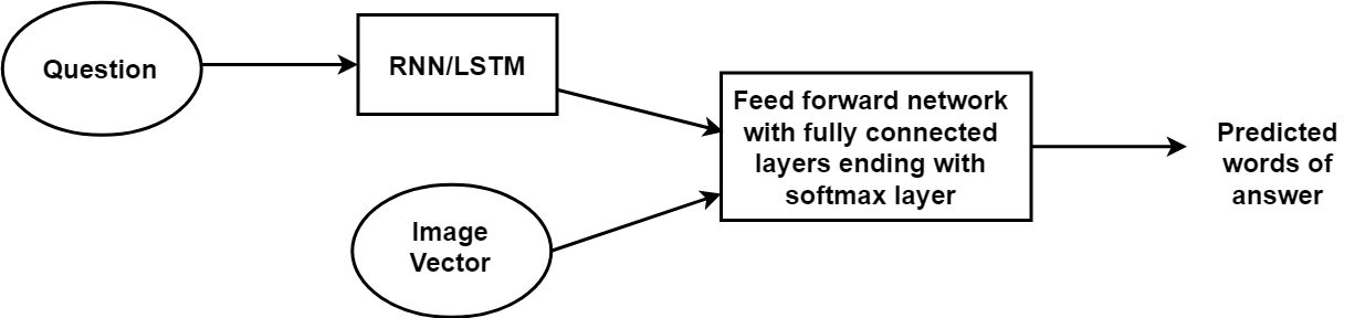
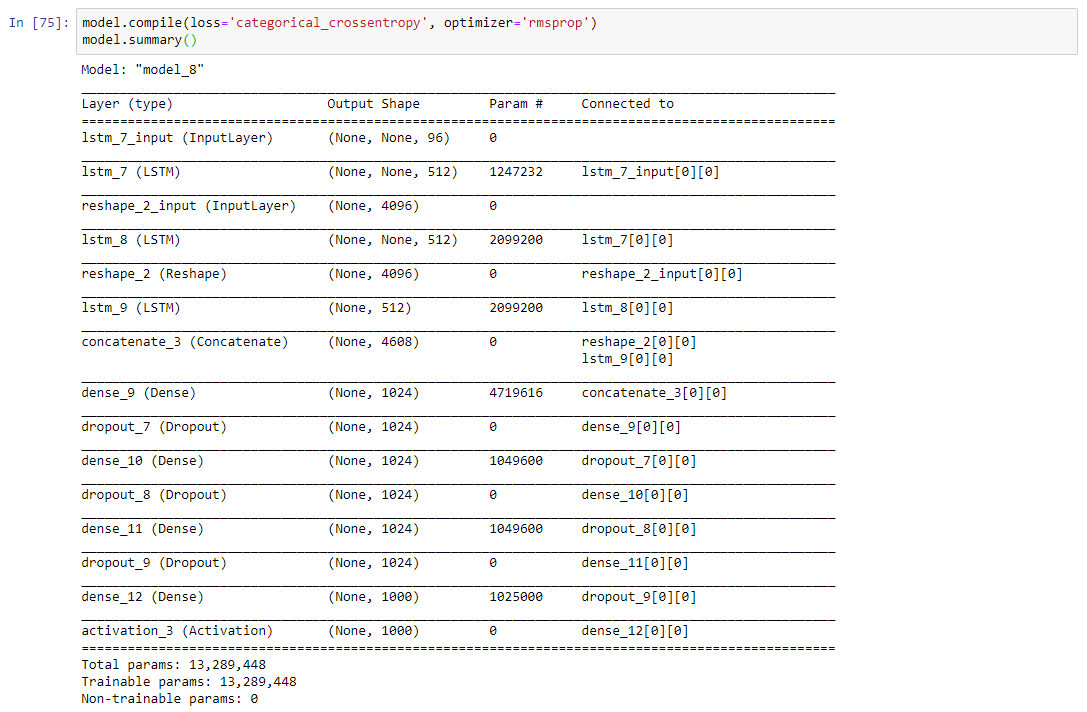
5. Model Architecture:

In our problem the input consists of two parts i.e an image vector, and a question, we cannot use the Sequential API of the Keras library. For this reason, we use the Functional API which allows us to create multiple models and finally merge models.

The below picture shows the high-level architecture idea of submodules of neural network.

After concatenating the 2 different models the summary will look like the following.

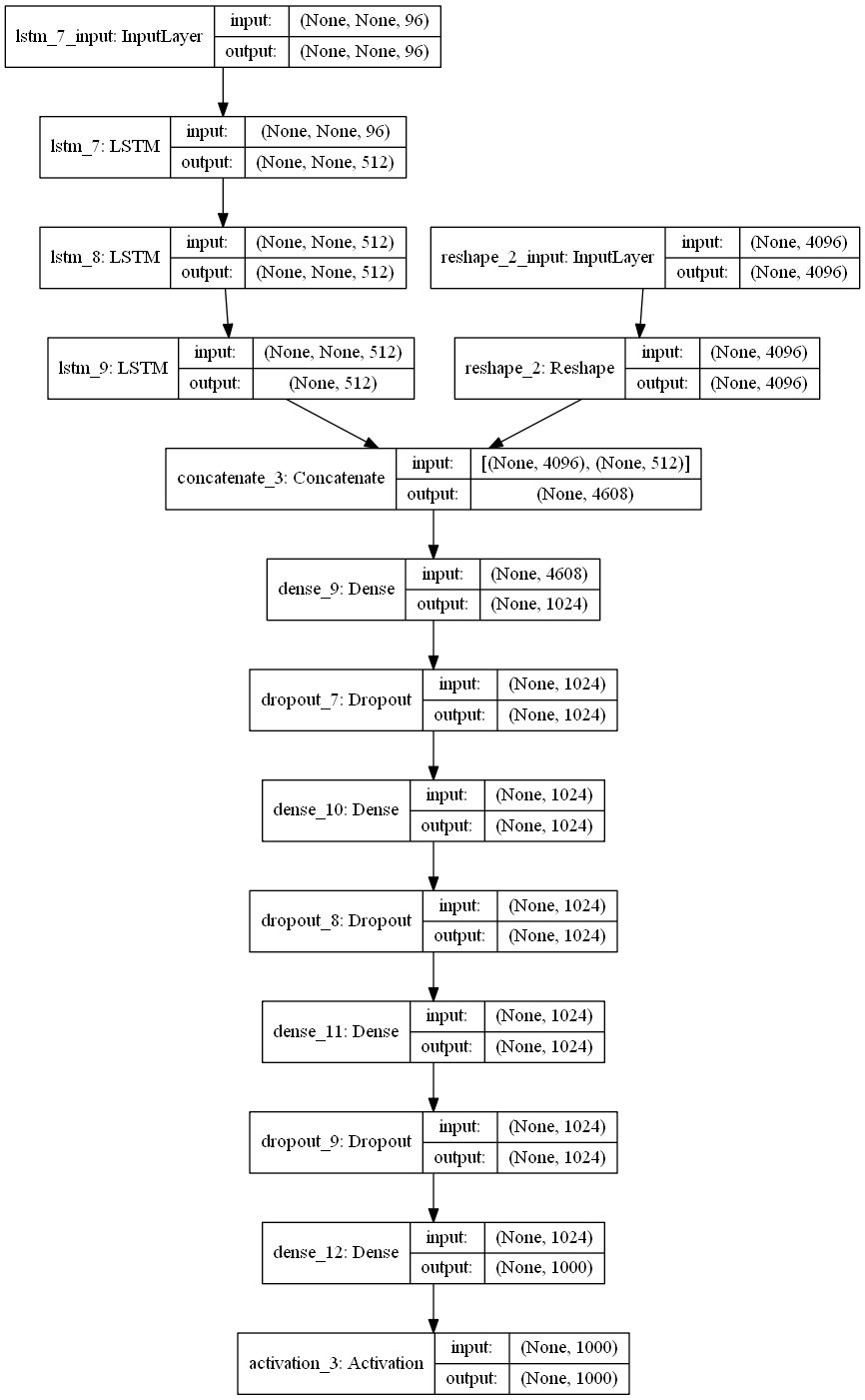
The below plot helps us to visualize neural network architecture and to understand the two types of input:


6. Defining model parameters:

The hyperparameters that we are going to use for our model is defined as follows:

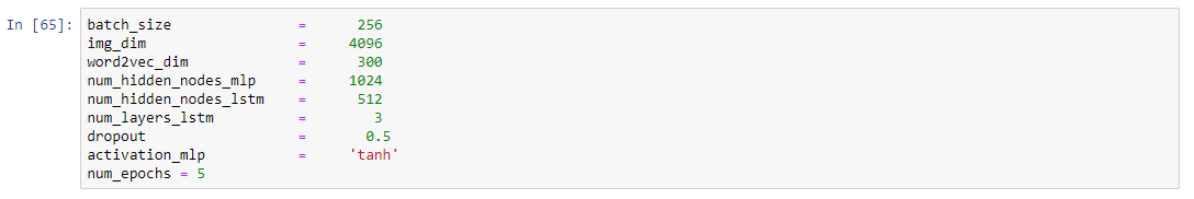
If you know what this parameter means then you can play around it and can get better results.

Time Taken: I used the GPU on https://colab.research.google.com and hence it took me approximately 2 hours to train the model for 5 epochs. However, if you train it on a PC without GPU, it could take more time depending on the configuration of your machine.

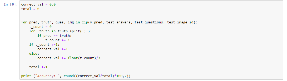
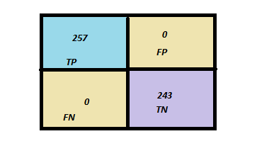
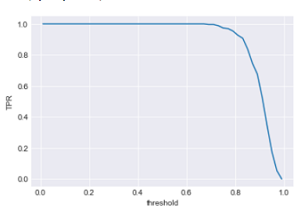
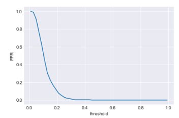
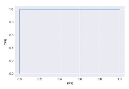
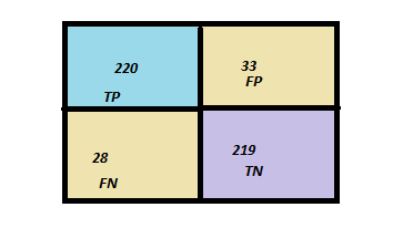
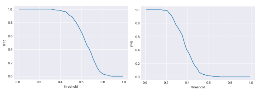
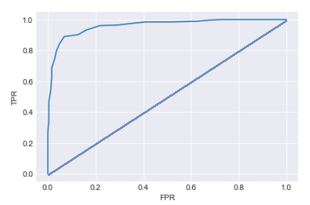
7. Evaluating the model:

Since I have used the very small dataset for performing these experiments I am not able to get very good accuracy. The below code will calculate the accuracy of the model.


Since I have trained a model multiple times with different parameters you will not get the same accuracy as me. If you want you can directly download mode.h5 file from my google drive.


8. Final Thoughts:

One of the interesting thing about VQA is that it a completely new field. So there is absolutely no end to what you can do to solve this problem. Below are some tips while replicating the code.

  1. Start with a very small subset of data: When you start implementing I suggest you start with a very small amount of data. Because once you are ready with the whole setup then you can scale it any time.
  2. Understand the code: Understanding code line by line is very much helpful to match your theoretical knowledge. So for that, I suggest you can take very few samples(maybe 20 or less) and run a small chunk (2 to 3 lines) of code to get the functionality of each part.
  3. Be patient: One of the mistakes that I did while starting with this project was to do everything at one go. If you get some error while replicating code spend 4 to 5 days harder on that. Even after that if you won’t able to solve, I would suggest you resume after a break of 1 or 2 days. 

VQA is the intersection of NLP and CV and hopefully, this project will give you a better understanding (more precisely practically) with most of the deep learning concepts.

If you want to improve the performance of the model below are few tips you can try:

  1. Use larger datasets
  2. Try Building more complex models like Attention, etc
  3. Try using other pre-trained word embeddings like Glove 
  4. Try using a different architecture 
  5. Do more hyperparameter tuning

The list is endless and it goes on.

In the blog, I have not provided the complete code you can get it from my Github repository.

9. References:

  1. https://blog.floydhub.com/asking-questions-to-images-with-deep-learning/
  2. https://tryolabs.com/blog/2018/03/01/introduction-to-visual-question-answering/
  3. https://github.com/sominwadhwa/vqamd_floyd

The Future of AI in Dental Technology

As we develop more advanced technology, we begin to learn that artificial intelligence can have more and more of an impact on our lives and industries that we have gotten used to being the same over the past decades. One of those industries is dentistry. In your lifetime, you’ve probably not seen many changes in technology, but a boom around artificial intelligence and technology has opened the door for AI in dental technologies.

How Can AI Help?

Though dentists take a lot of pride in their craft and career, most acknowledge that AI can do some things that they can’t do or would make their job easier if they didn’t have to do. AI can perform a number of both simple and advanced tasks. Let’s take a look at some areas that many in the dental industry feel that AI can be of assistance.

Repetitive, Menial Tasks

The most obvious area that AI can help out when it comes to dentistry is with repetitive and menial simple tasks. There are many administrative tasks in the dentistry industry that can be sped up and made more cost-effective with the use of AI. If we can train a computer to do some of these tasks, we may be able to free up more time for our dentists to focus on more important matters and improve their job performance as well. One primary use of AI is virtual consultations that offices like Philly Braces are offering. This saves patients time when they come in as the Doctor already knows what the next steps in their treatment will be.

Using AI to do some basic computer tasks is already being done on a small scale by some, but we have yet to see a very large scale implementation of this technology. We would expect that to happen soon, with how promising and cost-effective the technology has proven to be.

Reducing Misdiagnosis

One area that many think that AI can help a lot in is misdiagnosis. Though dentists do their best, there is still a nearly 20% misdiagnosis rate when reading x-rays in dentistry. We like to think that a human can read an x-ray better, but this may not be the case. AI technology can certainly be trained to read an x-ray and there have been some trials to suggest that they can do it better and identify key conditions that we often misread.

A world with AI diagnosis that is accurate and quicker will save time, money, and lead to better dental health among patients. It hasn’t yet come to fruition, but this seems to be the next major step for AI in dentistry.

Artificial Intelligence Assistants

Once it has been demonstrated that AI can perform a range of tasks that are useful to dentists, the next logical step is to combine those skills to make a fully-functional AI dental assistant. A machine like this has not yet been developed, but we can imagine that it would be an interface that could be spoken to similar to Alexa. The dentist would request vital information and other health history data from a patient or set of patients to assist in the treatment process. This would undoubtedly be a huge step forward and bring a lot of computing power into the average dentist office.

Conclusion

It’s clear that AI has a bright future in the dental industry and has already shown some of the essential skills that it can help with in order to provide more comprehensive and accurate care to dental patients. Some offices like Westwood Orthodontics already use AI in the form of a virtual consult to diagnose issues and provide treatment options before patients actually step foot in the office. Though not nearly all applications that AI can provide have been explored, we are well on our way to discovering the vast benefits of artificial intelligence for both patients and practices in the dental healthcare industry.

Accelerate your AI Skills Today: A Million Dollar Job!

The skyrocketing salaries ($1m per year) of AI engineers is not a hype. It is the fact of current corporate world, where you will witness a shift that is inevitable.

We’ve already set our feet at the edge of the technological revolution. A revolution that is at the verge of altering the way we live and work. As the fact suggests, humanity has fundamentally developed human production in three revolutions, and we’re now entering the fourth revolution. In its scope, the fourth revolution projects a transformation that is unlike anything we humans have ever experienced.

  • The first revolution had the world transformed from rural to urban
  • the emergence of mass production in the second revolution
  • third introduced the digital revolution
  • The fourth industrial revolution is anxious to integrate technologies into our lives.

And all thanks to artificial intelligence (AI). An advanced technology that surrounds us, from virtual assistants to software that translates to self-driving cars.

The rise of AI at an exponential rate has disrupted almost every industry. So much so that AI is being rated as one-million-dollar profession.

Did this grab your attention? It did?

Now, what if we were to tell you that the salary compensation for AI experts has grown dramatically. AI and machine learning are fields that have a mountain of demand in the tech industry today but has sparse supply.

AI field is growing at a quicker pace and salaries are skyrocketing! Read it for yourself to know what AI experts, AI researchers and any other AI talent are commanding today.

  • A top-class AI research laboratory, OpenAI says that techies in the AI field are projected to earn a salary compensation ranging between $300 to $500k for fresh graduates. However, expert professionals could earn anywhere up to $1m.
  • Whopping salary package of above 100 million yen that amounts to $1m is being offered to AI geniuses by a Japanese firm, Start Today. A firm that operates a fashion shopping website named Zozotown.

Does this leave you with a question – Is this a right opportunity for you to jump in the field and make hay while the sun is shining? 

And the answer to this question is – yes, it is the right opportunity for any developer seeking a role in the AI industry. It can be your chance to bridge the skill shortage in the AI field either by upskilling or reskilling yourself in the field of AI.

There are a wide varieties of roles available for an AI enthusiast like you. And certain areas are like AI Engineers and AI Researchers are high in demand, as there are not many professionals who have robust AI knowledge.

According to a job report, “The Future of Jobs 2018,” a prediction was made suggesting that machines and algorithms will create around 133 million new job roles by 2022.

AI and machine learning will dominate the tech world. The World Economic Forum says that several sectors have started embracing AI and machine learning to tackle challenges in certain fields such as advertising, supply chain, manufacturing, smart cities, drones, and cybersecurity.

Unraveling the AI realm

From chatbots to financial planners, AI is impacting the way businesses function on a day-today basis. AI makes the work simpler, as it provides variables, which makes the work more streamlined.

Alright! You know that

  • the demand for AI professionals is rising exponentially and that there is just a trickle of supply
  • the AI professionals are demanding skyrocketing salaries

However, beyond that how much more do you know about AI?

Considering the fact that our lives have already been touched by AI (think Alexa, and Siri), it is just a matter of time when AI will become an indispensable part of our lives.

As Gartner predicts that 2020 will be an important year for business growth in AI. Thus, it is possible to witness significant sparks for employment growth. Though AI predicts to diminish 1.8 million jobs, it is also said to replace it with 2.3 million jobs that will be created. As we look forward to stepping into 2020, AI-related job roles are set to make positive progress of achieving 2 million net-new employments by 2025.

With AI promising to score fat paychecks that would reach millions, AI experts are struggling to find new ways to pick up nouveau skills. However, one of the biggest impacts that affect the job market today is the scarcity of talent in this field.

The best way to stay relevant and employable in AI is probably by “reskilling,” and “upskilling.” And  AI certifications is considered ideal for those in the current workforce.

Looking to upskill yourself – here’s how you can become an AI engineer today.

Top three ways to enhance your artificial intelligence career:

  1. Acquire skills in Statistics and Machine Learning: If you’re getting into the field of machine learning, it is crucial that you have in-depth knowledge of statistics. Statistics is considered a prerequisite to the ML field. Both the fields are tightly related. Machine learning models are created to make accurate predictions while statistical models do the job of interpreting the relationship between variables. Many ML techniques heavily rely on the theory obtained through statistics. Thus, having extensive knowledge in statistics help initiate the first step towards an AI career.
  2. Online certification programs in AI skills: Opting for AI certifications will boost your credibility amongst potential employers. Certifications will also enhance your earning potential and increase your marketability. If you’re looking for a change and to be a part of something impactful; join the AI bandwagon. The IT industry is growing at breakneck speed; it is now that businesses are realizing how important it is to hire professionals with certain skillsets. Specifically, those who are certified in AI are becoming sought after in the job market.
  3. Hands-on experience: There’s a vast difference in theory and practical knowledge. One needs to familiarize themselves with the latest tools and technologies used by the industry. This is possible only if the individual is willing to work on projects and build things from scratch.

Despite all the promises, AI does prove to be a threat to job holders, if they don’t upskill or reskill themselves. The upcoming AI revolution will definitely disrupt the way we work, however, it will leave room for humans to perform more creative jobs in the future corporate world.

So a word of advice is to be prepared and stay future ready.

Visual Question Answering with Keras – Part 1

This is Part I of II of the Article Series Visual Question Answering with Keras

Making Computers Intelligent to answer from images

If we look closer in the history of Artificial Intelligence (AI), the Deep Learning has gained more popularity in the recent years and has achieved the human-level performance in the tasks such as Speech Recognition, Image Classification, Object Detection, Machine Translation and so on. However, as humans, not only we but also a five-year child can normally perform these tasks without much inconvenience. But the development of such systems with these capabilities has always considered an ambitious goal for the researchers as well as for developers.

In this series of blog posts, I will cover an introduction to something called VQA (Visual Question Answering), its available datasets, the Neural Network approach for VQA and its implementation in Keras and the applications of this challenging problem in real life. 

Table of Contents:

1 Introduction

2 What is exactly Visual Question Answering?

3 Prerequisites

4 Datasets available for VQA

4.1 DAQUAR Dataset

4.2 CLEVR Dataset

4.3 FigureQA Dataset

4.4 VQA Dataset

5 Real-life applications of VQA

6 Conclusion


  1. Introduction:

Let’s say you are given a below picture along with one question. Can you answer it?

I expect confidently you all say it is the Kitchen without much inconvenience which is also the right answer. Even a five-year child who just started to learn things might answer this question correctly.

Alright, but can you write a computer program for such type of task that takes image and question about the image as an input and gives us answer as output?

Before the development of the Deep Neural Network, this problem was considered as one of the difficult, inconceivable and challenging problem for the AI researcher’s community. However, due to the recent advancement of Deep Learning the systems are capable of answering these questions with the promising result if we have a required dataset.

Now I hope you have got at least some intuition of a problem that we are going to discuss in this series of blog posts. Let’s try to formalize the problem in the below section.

  1. What is exactly Visual Question Answering?:

We can define, “Visual Question Answering(VQA) is a system that takes an image and natural language question about the image as an input and generates natural language answer as an output.”

VQA is a research area that requires an understanding of vision(Computer Vision)  as well as text(NLP). The main beauty of VQA is that the reasoning part is performed in the context of the image. So if we have an image with the corresponding question then the system must able to understand the image well in order to generate an appropriate answer. For example, if the question is the number of persons then the system must able to detect faces of the persons. To answer the color of the horse the system need to detect the objects in the image. Many of these common problems such as face detection, object detection, binary object classification(yes or no), etc. have been solved in the field of Computer Vision with good results.

To summarize a good VQA system must be able to address the typical problems of CV as well as NLP.

To get a better feel of VQA you can try online VQA demo by CloudCV. You just go to this link and try uploading the picture you want and ask the related question to the picture, the system will generate the answer to it.


  1. Prerequisites:

In the next post, I will walk you through the code for this problem using Keras. So I assume that you are familiar with:

  1. Fundamental concepts of Machine Learning
  2. Multi-Layered Perceptron
  3. Convolutional Neural Network
  4. Recurrent Neural Network (especially LSTM)
  5. Gradient Descent and Backpropagation
  6. Transfer Learning
  7. Hyperparameter Optimization
  8. Python and Keras syntax
  1. Datasets available for VQA:

As you know problems related to the CV or NLP the availability of the dataset is the key to solve the problem. The complex problems like VQA, the dataset must cover all possibilities of questions answers in real-world scenarios. In this section, I will cover some of the datasets available for VQA.

4.1 DAQUAR Dataset:

The DAQUAR dataset is the first dataset for VQA that contains only indoor scenes. It shows the accuracy of 50.2% on the human baseline. It contains images from the NYU_Depth dataset.

Example of DAQUAR dataset

Example of DAQUAR dataset

The main disadvantage of DAQUAR is the size of the dataset is very small to capture all possible indoor scenes.

4.2 CLEVR Dataset:

The CLEVR Dataset from Stanford contains the questions about the object of a different type, colors, shapes, sizes, and material.

It has

  • A training set of 70,000 images and 699,989 questions
  • A validation set of 15,000 images and 149,991 questions
  • A test set of 15,000 images and 14,988 questions

Image Source: https://cs.stanford.edu/people/jcjohns/clevr/?source=post_page


4.3 FigureQA Dataset:

FigureQA Dataset contains questions about the bar graphs, line plots, and pie charts. It has 1,327,368 questions for 100,000 images in the training set.

4.4 VQA Dataset:

As comapred to all datasets that we have seen so far VQA dataset is relatively larger. The VQA dataset contains open ended as well as multiple choice questions. VQA v2 dataset contains:

  • 82,783 training images from COCO (common objects in context) dataset
  • 40, 504 validation images and 81,434 validation images
  • 443,757 question-answer pairs for training images
  • 214,354 question-answer pairs for validation images.

As you might expect this dataset is very huge and contains 12.6 GB of training images only. I have used this dataset in the next post but a very small subset of it.

This dataset also contains abstract cartoon images. Each image has 3 questions and each question has 10 multiple choice answers.

  1. Real-life applications of VQA:

There are many applications of VQA. One of the famous applications is to help visually impaired people and blind peoples. In 2016, Microsoft has released the “Seeing AI” app for visually impaired people to describe the surrounding environment around them. You can watch this video for the prototype of the Seeing AI app.

Another application could be on social media or e-commerce sites. VQA can be also used for educational purposes.

  1. Conclusion:

I hope this explanation will give you a good idea of Visual Question Answering. In the next blog post, I will walk you through the code in Keras.

If you like my explanations, do provide some feedback, comments, etc. and stay tuned for the next post.

A Bird’s Eye View: How Machine Learning Can Help You Charge Your E-Scooters

Bird scooters in Columbus, Ohio

Bird scooters in Columbus, Ohio

Ever since I started using bike-sharing to get around in Seattle, I have become fascinated with geolocation data and the transportation sharing economy. When I saw this project leveraging the mobility data RESTful API from the Los Angeles Department of Transportation, I was eager to dive in and get my hands dirty building a data product utilizing a company’s mobility data API.

Unfortunately, the major bike and scooter providers (Bird, JUMP, Lime) don’t have publicly accessible APIs. However, some folks have seemingly been able to reverse-engineer the Bird API used to populate the maps in their Android and iOS applications.

One interesting feature of this data is the nest_id, which indicates if the Bird scooter is in a “nest” — a centralized drop-off spot for charged Birds to be released back into circulation.

I set out to ask the following questions:

  1. Can real-time predictions be made to determine if a scooter is currently in a nest?
  2. For non-nest scooters, can new nest location recommendations be generated from geospatial clustering?

To answer these questions, I built a full-stack machine learning web application, NestGenerator, which provides an automated recommendation engine for new nest locations. This application can help power Bird’s internal nest location generation that runs within their Android and iOS applications. NestGenerator also provides real-time strategic insight for Bird chargers who are enticed to optimize their scooter collection and drop-off route based on proximity to scooters and nest locations in their area.

Bird

The electric scooter market has seen substantial growth with Bird’s recent billion dollar valuation  and their $300 million Series C round in the summer of 2018. Bird offers electric scooters that top out at 15 mph, cost $1 to unlock and 15 cents per minute of use. Bird scooters are in over 100 cities globally and they announced in late 2018 that they eclipsed 10 million scooter rides since their launch in 2017.

Bird scooters in Tel Aviv, Israel

Bird scooters in Tel Aviv, Israel

With all of these scooters populating cities, there’s much-needed demand for people to charge them. Since they are electric, someone needs to charge them! A charger can earn additional income for charging the scooters at their home and releasing them back into circulation at nest locations. The base price for charging each Bird is $5.00. It goes up from there when the Birds are harder to capture.

Data Collection and Machine Learning Pipeline

The full data pipeline for building “NestGenerator”

Data

From the details here, I was able to write a Python script that returned a list of Bird scooters within a specified area, their geolocation, unique ID, battery level and a nest ID.

I collected scooter data from four cities (Atlanta, Austin, Santa Monica, and Washington D.C.) across varying times of day over the course of four weeks. Collecting data from different cities was critical to the goal of training a machine learning model that would generalize well across cities.

Once equipped with the scooter’s latitude and longitude coordinates, I was able to leverage additional APIs and municipal data sources to get granular geolocation data to create an original scooter attribute and city feature dataset.

Data Sources:

  • Walk Score API: returns a walk score, transit score and bike score for any location.
  • Google Elevation API: returns elevation data for all locations on the surface of the earth.
  • Google Places API: returns information about places. Places are defined within this API as establishments, geographic locations, or prominent points of interest.
  • Google Reverse Geocoding API: reverse geocoding is the process of converting geographic coordinates into a human-readable address.
  • Weather Company Data: returns the current weather conditions for a geolocation.
  • LocationIQ: Nearby Points of Interest (PoI) API returns specified PoIs or places around a given coordinate.
  • OSMnx: Python package that lets you download spatial geometries and model, project, visualize, and analyze street networks from OpenStreetMap’s APIs.

Feature Engineering

After extensive API wrangling, which included a four-week prolonged data collection phase, I was finally able to put together a diverse feature set to train machine learning models. I engineered 38 features to classify if a scooter is currently in a nest.

Full Feature Set

Full Feature Set

The features boiled down into four categories:

  • Amenity-based: parks within a given radius, gas stations within a given radius, walk score, bike score
  • City Network Structure: intersection count, average circuity, street length average, average streets per node, elevation level
  • Distance-based: proximity to closest highway, primary road, secondary road, residential road
  • Scooter-specific attributes: battery level, proximity to closest scooter, high battery level (> 90%) scooters within a given radius, total scooters within a given radius


Log-Scale Transformation

For each feature, I plotted the distribution to explore the data for feature engineering opportunities. For features with a right-skewed distribution, where the mean is typically greater than the median, I applied these log transformations to normalize the distribution and reduce the variability of outlier observations. This approach was used to generate a log feature for proximity to closest scooter, closest highway, primary road, secondary road, and residential road.

An example of a log transformation

Statistical Analysis: A Systematic Approach

Next, I wanted to ensure that the features I included in my model displayed significant differences when broken up by nest classification. My thinking was that any features that did not significantly differ when stratified by nest classification would not have a meaningful predictive impact on whether a scooter was in a nest or not.

Distributions of a feature stratified by their nest classification can be tested for statistically significant differences. I used an unpaired samples t-test with a 0.01% significance level to compute a p-value and confidence interval to determine if there was a statistically significant difference in means for a feature stratified by nest classification. I rejected the null hypothesis if a p-value was smaller than the 0.01% threshold and if the 99.9% confidence interval did not straddle zero. By rejecting the null-hypothesis in favor of the alternative hypothesis, it’s deemed there is a significant difference in means of a feature by nest classification.

Battery Level Distribution Stratified by Nest Classification to run a t-test

Battery Level Distribution Stratified by Nest Classification to run a t-test

Log of Closest Scooter Distribution Stratified by Nest Classification to run a t-test

Throwing Away Features

Using the approach above, I removed ten features that did not display statistically significant results.

Statistically Insignificant Features Removed Before Model Development

Model Development

I trained two models, a random forest classifier and an extreme gradient boosting classifier since tree-based models can handle skewed data, capture important feature interactions, and provide a feature importance calculation. I trained the models on 70% of the data collected for all four cities and reserved the remaining 30% for testing.

After hyper-parameter tuning the models for performance on cross-validation data it was time to run the models on the 30% of test data set aside from the initial data collection.

I also collected additional test data from other cities (Columbus, Fort Lauderdale, San Diego) not involved in training the models. I took this step to ensure the selection of a machine learning model that would generalize well across cities. The performance of each model on the additional test data determined which model would be integrated into the application development.

Performance on Additional Cities Test Data

The Random Forest Classifier displayed superior performance across the board

The Random Forest Classifier displayed superior performance across the board

I opted to move forward with the random forest model because of its superior performance on AUC score and accuracy metrics on the additional cities test data. AUC is the Area under the ROC Curve, and it provides an aggregate measure of model performance across all possible classification thresholds.

AUC Score on Test Data for each Model

AUC Score on Test Data for each Model

Feature Importance

Battery level dominated as the most important feature. Additional important model features were proximity to high level battery scooters, proximity to closest scooter, and average distance to high level battery scooters.

Feature Importance for the Random Forest Classifier

Feature Importance for the Random Forest Classifier

The Trade-off Space

Once I had a working machine learning model for nest classification, I started to build out the application using the Flask web framework written in Python. After spending a few days of writing code for the application and incorporating the trained random forest model, I had enough to test out the basic functionality. I could finally run the application locally to call the Bird API and classify scooter’s into nests in real-time! There was one huge problem, though. It took more than seven minutes to generate the predictions and populate in the application. That just wasn’t going to cut it.

The question remained: will this model deliver in a production grade environment with the goal of making real-time classifications? This is a key trade-off in production grade machine learning applications where on one end of the spectrum we’re optimizing for model performance and on the other end we’re optimizing for low latency application performance.

As I continued to test out the application’s performance, I still faced the challenge of relying on so many APIs for real-time feature generation. Due to rate-limiting constraints and daily request limits across so many external APIs, the current machine learning classifier was not feasible to incorporate into the final application.

Run-Time Compliant Application Model

After going back to the drawing board, I trained a random forest model that relied primarily on scooter-specific features which were generated directly from the Bird API.

Through a process called vectorization, I was able to transform the geolocation distance calculations utilizing NumPy arrays which enabled batch operations on the data without writing any “for” loops. The distance calculations were applied simultaneously on the entire array of geolocations instead of looping through each individual element. The vectorization implementation optimized real-time feature engineering for distance related calculations which improved the application response time by a factor of ten.

Feature Importance for the Run-time Compliant Random Forest Classifier

Feature Importance for the Run-time Compliant Random Forest Classifier

This random forest model generalized well on test-data with an AUC score of 0.95 and an accuracy rate of 91%. The model retained its prediction accuracy compared to the former feature-rich model, but it gained 60x in application performance. This was a necessary trade-off for building a functional application with real-time prediction capabilities.

Geospatial Clustering

Now that I finally had a working machine learning model for classifying nests in a production grade environment, I could generate new nest locations for the non-nest scooters. The goal was to generate geospatial clusters based on the number of non-nest scooters in a given location.

The k-means algorithm is likely the most common clustering algorithm. However, k-means is not an optimal solution for widespread geolocation data because it minimizes variance, not geodetic distance. This can create suboptimal clustering from distortion in distance calculations at latitudes far from the equator. With this in mind, I initially set out to use the DBSCAN algorithm which clusters spatial data based on two parameters: a minimum cluster size and a physical distance from each point. There were a few issues that prevented me from moving forward with the DBSCAN algorithm.

  1. The DBSCAN algorithm does not allow for specifying the number of clusters, which was problematic as the goal was to generate a number of clusters as a function of non-nest scooters.
  2. I was unable to hone in on an optimal physical distance parameter that would dynamically change based on the Bird API data. This led to suboptimal nest locations due to a distortion in how the physical distance point was used in clustering. For example, Santa Monica, where there are ~15,000 scooters, has a higher concentration of scooters in a given area whereas Brookline, MA has a sparser set of scooter locations.

An example of how sparse scooter locations vs. highly concentrated scooter locations for a given Bird API call can create cluster distortion based on a static physical distance parameter in the DBSCAN algorithm. Left:Bird scooters in Brookline, MA. Right:Bird scooters in Santa Monica, CA.

An example of how sparse scooter locations vs. highly concentrated scooter locations for a given Bird API call can create cluster distortion based on a static physical distance parameter in the DBSCAN algorithm. Left:Bird scooters in Brookline, MA. Right:Bird scooters in Santa Monica, CA.

Given the granularity of geolocation scooter data I was working with, geospatial distortion was not an issue and the k-means algorithm would work well for generating clusters. Additionally, the k-means algorithm parameters allowed for dynamically customizing the number of clusters based on the number of non-nest scooters in a given location.

Once clusters were formed with the k-means algorithm, I derived a centroid from all of the observations within a given cluster. In this case, the centroids are the mean latitude and mean longitude for the scooters within a given cluster. The centroids coordinates are then projected as the new nest recommendations.

NestGenerator showcasing non-nest scooters and new nest recommendations utilizing the K-Means algorithm

NestGenerator showcasing non-nest scooters and new nest recommendations utilizing the K-Means algorithm.

NestGenerator Application

After wrapping up the machine learning components, I shifted to building out the remaining functionality of the application. The final iteration of the application is deployed to Heroku’s cloud platform.

In the NestGenerator app, a user specifies a location of their choosing. This will then call the Bird API for scooters within that given location and generate all of the model features for predicting nest classification using the trained random forest model. This forms the foundation for map filtering based on nest classification. In the app, a user has the ability to filter the map based on nest classification.

Drop-Down Map View filtering based on Nest Classification

Drop-Down Map View filtering based on Nest Classification

Nearest Generated Nest

To see the generated nest recommendations, a user selects the “Current Non-Nest Scooters & Predicted Nest Locations” filter which will then populate the application with these nest locations. Based on the user’s specified search location, a table is provided with the proximity of the five closest nests and an address of the Nest location to help inform a Bird charger in their decision-making.

NestGenerator web-layout with nest addresses and proximity to nearest generated nests

NestGenerator web-layout with nest addresses and proximity to nearest generated nests

Conclusion

By accurately predicting nest classification and clustering non-nest scooters, NestGenerator provides an automated recommendation engine for new nest locations. For Bird, this application can help power their nest location generation that runs within their Android and iOS applications. NestGenerator also provides real-time strategic insight for Bird chargers who are enticed to optimize their scooter collection and drop-off route based on scooters and nest locations in their area.

Code

The code for this project can be found on my GitHub

Comments or Questions? Please email me an E-Mail!


Introduction to ROC Curve

The abbreviation ROC stands for Receiver Operating Characteristic. Its main purpose is to illustrate the diagnostic ability of classifier as the discrimination threshold is varied. It was developed during World War II when Radar operators had to decide if the blip on the screen is an enemy target, a friendly ship or just a noise.  For these purposes they measured the ability of a radar receiver operator to make these important distinctions, which was called the Receiver Operating Characteristic.

Later it was found useful in interpreting medical test results and then in Machine learning classification problems. In order to get an introduction to binary classification and terms like ‘precision’ and ‘recall’ one can look into my earlier blog  here.

True positive rate and false positive rate

Let’s imagine a situation where a fire alarm is installed in a kitchen. The alarm is supposed to emit a sound in case fire smoke is detected in the room. Unfortunately, there is a lot of cooking done in the kitchen and the alarm may trigger the sound too often. Thus, instead of serving a purpose the alarm becomes a nuisance due to a large number of false alarms. In statistical terms these types of errors are called type 1 errors, or false positives.

One way to deal with this problem is to simply decrease sensitivity of the device. We do this by increasing the trigger threshold at the alarm setting. But then, not every alarm should have the same threshold setting. Consider the same type of device but kept in a bedroom. With high threshold, the device might miss smoke from a real short-circuit in the wires which poses a real danger of fire. This kind of failure is called Type 2 error or a false negative. Although the two devices are the same, different types of threshold settings are optimal for different circumstances.

To specify this more formally, let us describe the performance of a binary classifier at a particular threshold by the following parameters:


These parameters take different values at different thresholds. Hence, they define the performance of the classifier at particular threshold. But we want to examine in overall how good a classifier is. Fortunately, there is a way to do that. We plot the True Positive Rate (TPR) and False Positive rate (FPR) at different thresholds and this plot is called ROC curve.

Let’s try to understand this with an example.

A case with a distinct population distribution

Let’s suppose there is a disease which can be identified with deficiency of some parameter (maybe a certain vitamin). The distribution of population with this disease has a mean vitamin concentration sharply distinct from the mean of a healthy population, as shown below.

This is result of dummy data simulating population of 2000 people,the link to the code is given  in the end of this blog.  As the two populations are distinctly separated (there is no  overlap between the two distributions), we can expect that a classifier would have an easy job distinquishing healthy from sick people. We can run a logistic regression classifier with a threshold of .5 and be 100% succesful in detecting the decease.

The confusion matrix may look something like this.

In this ideal case with a threshold  of  .5 we do not make a single wrong classification. The True positive rate and False positive rate are 1 and 0, respectively. But we can shift the threshold. In that case, we will  get different confusion matrices. First we plot threshold vs. TPR.

We see for most values of threshold the TPR is close to 1 which again proves data is easy to classify and the classifier is returning high probabilities  for the most of positives .

Similarly Let’s plot threshold vs. FPR.

For most of the data points FPR is close to zero. This is also good. Now its time to plot the ROC curve using these results (TPR vs FPR).

Let’s try to interpret  the results,  all the points lie on line x=0 and y=1, it means for all the points FPR is zero or TPR is one, making  the curve a square. which means the classifier does perfectly well.

Case with overlapping  population distribution

The above example was about a perfect classifer. However, life is often not so easy. Now let us consider another more realistic situation in which the parameter distribution of the population is not as distinct as in the previous case. Rather, the mean of the parameter with healthy and not healthy datapoints are close and the distributions overlap, as shown in the next figure.

If we set the threshold to 0.5, the confusion matrix may look like this.

Now, any new choice of threshold location will affect both false positives and false negatives. In fact, there is a trade-off. If we shift the threshold with the goal to reduce false negatives, false positives will increase. If we move the threshold to the other direction and reduce false positive, false negatives will increase.

The plots (TPR vs Threshold) , (FPR vs Threshold) are shown below

If we plot the ROC curve from these results, it looks like this:

From the curve we see the classifier does not perform as well as the earlier one.

What else can be infered from this curve? We first need to understand what the diagonal in this plot represent. The diagonal represents ‘Line of no discrimination’, which we obtain if we randomly guess. This is the ROC curve for the worst possible classifier. Therefore, by comparing the obtained ROC curve with the diagonal, we see how much better our classifer is from random guessing.

The further away ROC curve from the diagonal is (the closest it is to the top left corner) , better the classifier is.

Area Under the curve

The overall performance of the classifier is given by the area under the ROC curve and is usually denoted as AUC. Since TPR and FPR lie within the range of 0 to 1, the AUC also assumes values between 0 and 1. The higher the value of AUC, the better is the overall performance of the classifier.

Let’s see this for the two different distributions which we saw earlier.

As we know the classifier had worked perfectly in the first case with points at (0,1) the area under the curve is 1 which is perfect. In the latter case the classifier was not able to perform as good, the ROC curve is between the diagonal and left hand corner. The AUC as we can see is less than 1.

Some other general characteristics

There are still few points that needs to be discussed on a General ROC curve

  • The ROC curve does not provide information about the actual values of thresholds used for the classifier.
  • Performance of different classifiers can be compared using the AUC of different Classifier. The larger the AUC, the better the classifier.
  • The vertical distance of the ROC curve from the no discrimination line gives a measure of ‘INFORMEDNESS’. This is known as Youden’s J satistic. This statistics can take values between 0 and 1.

Youden’s  J statistic is defined for every point on the ROC curve . The point at which Youden’s  J satistics reaches its maximum for a given ROC curve can be used to guide the selection of the threshold to be used for that classifier.

I hope this post does the job of providing an understanding of ROC curves  and AUC. The  Python program for simulating the example given earlier can be found here .

Please feel free to adjust the mean of the distributions and see the changes in the plot.

How is automation changing data science and machine learning?

We have come a long way since the introduction of data science and machine learning. The recent study has found that the volume of business data doubles in less than 14 months. Today, the collection of data is no longer a problem, but the filtration, analysis, and maintenance of relevant information is a bigger issue.

We need to hire data science professionals, and they demand over $100k annually. Paying that sort of money for a professional is not feasible for every single organization, especially small and middle-sized companies. Google recently announced that it is going to make machine learning technology possible for every business.

The access to machine learning technology is now possible, even for small businesses due to automation. Google, Microsoft, and other companies have come up with automated machine learning tools that enable small businesses to use machine learning technology to enhance their business performance and profit.

Image Source: Google Cloud

With that said, the world still needs a lot of machine learning professionals. Many machine learning professionals prefer Python for machine learning due to its features and a wide range of libraries.

According to the Gartner report, around 40% of data science tasks will be automated by 2020. The data science tools can automate some parts of data science processes, but it is not complete automation.

With that said, it has been helping a lot to accelerate the tasks. We still need data science professionals to deal with real-world problems. The algorithms are not yet able to handle messy data. The significant chunk of data science professionals often prefers performing with data science with Python for sophisticated tasks.

Automation in Data Science

Let me show you the figure right at the beginning before moving forward.

Image Source: Wikipedia

If I had to use only one word to describe the entire data science process, I would use the word “headache.” According to the recent report, the median salary of data scientists easily surpasses $100k annually. The pay will be higher in the time to come.

One needs to pay a lot of money and invest a lot of time to get insights from the collected data. The data scientists need to spend almost 50-60% of their time in data processing and the rest of their time in modeling and deployment.

The cloud platforms like Amazon Web Services, Google, Microsoft Azure, and so on make the job more comfortable, but there is still a lot of work to maintain and extract useful insights from the collected data.

The data science process has lots of inefficiencies. At first, they need to spend over 50% of their total time on processing messy real-world data. After that, there could be a need to customize models, according to specific problems.

The significant contribution of automation is making a significant portion of data processing parts automated. Secondly, the automated platforms can make tracking of various models easier from multiple parameters. The time needed to launch the algorithm is minimal.

One example of an extensive tool to handle a data science project is Alteryx. IT has come up with powerful automated solutions that can drastically reduce the data processing and model development time for smoothening the entire data science workflow. The data science platform, Alteryx, is so amazing that its share price doubled in a span of little more than a year.

Some other great tools that can help you in data science automation are Rapidminer, H20.ai, KNIME, and so on. However, the lack of skilled data scientists can create a problem despite these tools. It is where the role of automated machine learning pops in.

How is Machine Learning Transformed with the entrance of Automation?

The traditional machine learning process was too complicated. One requires to have a lot of expensive machine learning professionals working for months to come up with models to process machine learning tasks.

Image Source: Medium

To make traditional machine learning work, one needs to gather data, standardize data, process features, create and train the machine learning model from problems, validate the models, and deploy the models at last.

You must have heard of how machine learning is only for corporations in the past. But, that has drastically changed in recent time, and it is all due to automation. Keep in mind that the above machine learning model is a simple one. There is a lot of extra works for complicated models. Even for the simple ones, you need to spend a lot of time and money, which makes it impossible for small and medium companies.

The automation in machine learning is all about automating the entire process to make machine learning easier. The only thing you need to do is feed data to the system (not a massive volume of data). You do not need even to cross the three-figure number of images to continue with automated machine learning platforms.

Microsoft has its automl platform along with Google. Other automl platforms can do the trick for you. Using those platforms do not cost you an arm and a leg. If you check out the price, you will be surprised.

There is no need for you to create or deploy models or even test the models. The algorithm will do the job for you. It takes examples and models of historical models to process the data and use a machine learning algorithm.

Even non-statistician can implement machine learning technology with limited data, thanks to automation in machine learning. You can make use of predictive analytics and can get easy solutions for simple prediction problems without scratching your head. Numerous libraries can assist you in the automated generation of machine learning pipelines.

How are the jobs of data scientists simplified by the introduction of automation in machine learning and data science?

It is true that the introduction of automation has drastically reduced the time for completing the tasks for data scientists. They no longer have to spend their valuable time in time-consuming, monotonous works that are necessary but do not provide a lot of value.

However, the need for skilled data scientists still exist, and it will always be there in the time to come. There are challenging works for data scientists that we cannot replace with machines, such as listening to clients, figuring out the root cause of business issues, development and selection of the right solution for the specific business problem.

Just like in other types of jobs, the advancement of automation technologies will modify the tasks that data scientists need to perform. They will be able to allocate more time on things that matter rather than monotonous tasks.

Final Verdict

The automation of machine learning and data science are in the beginning stage. However, they are already making a massive impact on the business world. The huge corporations are investing in Big Data and Machine Learning technologies. We can expect a considerable improvement in these technologies shortly.

Sooner, the competitive advantage of a business will depend on how well they can use the technologies, instead of access to machine learning or Big Data technologies.  I hope this article was valuable to you. If you want to add something or express your thoughts, feel free to leave a comment. I will gladly read and reply to your comment.

Fehler-Rückführung mit der Backpropagation

Dies ist Artikel 4 von 6 der Artikelserie –Einstieg in Deep Learning.

Das Gradienten(abstiegs)verfahren ist der Schlüssel zum Training einzelner Neuronen bzw. deren Gewichtungen zu den Neuronen der vorherigen Schicht. Wer dieses Prinzip verstanden hat, hat bereits die halbe Miete zum Verständnis des Trainings von künstlichen neuronalen Netzen.

Der Gradientenabstieg wird häufig fälschlicherweise mit der Backpropagation gleichgesetzt, jedoch ist das nicht ganz richtig, denn die Backpropagation ist mehr als die Anwendung des Gradientenabstiegs.

Bevor wir die Backpropagation erläutern, nochmal kurz zurück zur Forward-Propagation, die die eigentliche Prädiktion über ein künstliches neuronales Netz darstellt:

Forward-Propagation

Abbildung 1: Ein simples kleines künstliches neuronales Netz mit zwei Schichten (+ Eingabeschicht) und zwei Neuronen pro Schicht.

In einem kleinen künstlichen neuronalen Netz, wie es in der Abbildung 1 dargestellt ist, und das alle Neuronen über die Sigmoid-Funktion aktiviert, wird jedes Neuron eine Nettoeingabe z berechnen…

z = w^{T} \cdot x

… und diese Nettoeingabe in die Sigmoid-Funktion einspeisen…

\phi(z) = sigmoid(z) = \frac{1}{1 + e^{-z}}

… die dann das einzelne Neuron aktiviert. Die Aktivierung erfolgt also in der mittleren Schicht (N-Schicht) wie folgt:

N_{j} = \frac{1}{1 + e^{- \sum (w_{ij} \cdot x_{i}) }}

Die beiden Aktivierungsausgaben N werden dann als Berechnungsgrundlage für die Ausgaben der Ausgabeschicht o verwendet. Auch die Ausgabe-Neuronen berechnen ihre jeweilige Nettoeingabe z und aktivieren über Sigmoid(z).

Ausgabe eines Ausgabeknotens als Funktion der Eingänge und der Verknüpfungsgewichte für ein dreischichtiges neuronales Netz, mit nur zwei Knoten je Schicht, kann also wie folgt zusammen gefasst werden:

O_{k} = \frac{1}{1 + e^{- \sum (w_{jk} \cdot \frac{1}{1 + e^{- \sum (w_{ij} \cdot x_{i}) }}) }}

Abbildung 2: Forward-Propagation. Aktivierung via Sigmoid-Funktion.

Sollte dies die erste Forward-Propagation gewesen sein, wird der Output noch nicht auf den Input abgestimmt sein. Diese Abstimmung erfolgt in Form der Gewichtsanpassung im Training des neuronalen Netzes, über die zuvor erwähnte Gradientenmethode. Die Gradientenmethode ist jedoch von einem Fehler abhängig. Diesen Fehler zu bestimmen und durch das Netz zurück zu führen, das ist die Backpropagation.

Back-Propagation

Um die Gewichte entgegen des Fehlers anpassen zu können, benötigen wir einen möglichst exakten Fehler als Eingabe. Der Fehler berechnet sich an der Ausgabeschicht über eine Fehlerfunktion (Loss Function), beispielsweise über den MSE (Mean Squared Error) oder über die sogenannte Kreuzentropie (Cross Entropy). Lassen wir es in diesem Beispiel einfach bei einem simplen Vergleich zwischen dem realen Wert (Sollwert o_{real}) und der Prädiktion (Ausgabe o) bleiben:

e_{o} = o_{real} - o

Der Fehler e ist also einfach der Unterschied zwischen dem Ziel-Wert und der Prädiktion. Jedes Training ist eine Wiederholung von Prädiktion (Forward) und Gewichtsanpassung (Back). Im ersten Schritt werden üblicherweise die Gewichtungen zufällig gesetzt, jede Gewichtung unterschiedlich nach Zufallszahl. So ist die Wahrscheinlichkeit, gleich zu Beginn die “richtigen” Gewichtungen gefunden zu haben auch bei kleinen neuronalen Netzen verschwindend gering. Der Fehler wird also groß sein und kann über den Gradientenabstieg durch Gewichtsanpassung verkleinert werden.

In diesem Beispiel berechnen wir die Fehler e_{1} und e_{2} und passen danach die Gewichte w_{j,k} (w_{1,1} & w_{2,1} und w_{1,2} & w_{2,2}) der Schicht zwischen dem Hidden-Layer N und dem Output-Layer o an.

Abbildung 3: Anpassung der Gewichtungen basierend auf dem Fehler in der Ausgabe-Schicht.

Die Frage ist nun, wie die Gewichte zwischen dem Input-Layer X 
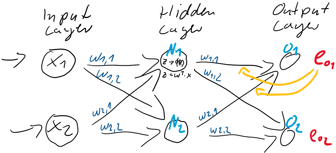
und dem Hidden-Layer N anzupassen sind. Es stellt sich die Frage, welchen Einfluss diese auf die Fehler in der Ausgabe-Schicht haben?

Um diese Gewichtungen anpassen zu können, benötigen wir den Fehler-Anteil der beiden Neuronen N_{1} und N_{2}. Dieser Anteil am Fehler der jeweiligen Neuronen ergibt sich direkt aus den Gewichtungen w_{j,k} zum Output-Layer:

e_{N_{1}} = e_{o1} \cdot \frac{w_{1,1}}{w_{1,1} + w_{1,2}} + e_{o2} \cdot \frac{w_{1,2}}{w_{1,1} + w_{1,2}}

e_{N_{2}} = e_{o1} \cdot \frac{w_{2,1}}{w_{2,1} + w_{2,2}} + e_{o2} \cdot \frac{w_{2,2}}{w_{2,1} + w_{2,2}}

Wenn man das nun generalisiert:

    \[ e_{N} = \left(\begin{array}{rr} \frac{w_{1,1}}{w_{1,1} + w_{1,2}} & \frac{w_{1,2}}{w_{1,1} + w_{1,2}} \\ \frac{w_{2,1}}{w_{2,1} + w_{2,2}} & \frac{w_{2,2}}{w_{2,1} + w_{2,2}} \end{array}\right) \cdot \left(\begin{array}{c} e_{1} \\ e_{2} \end{array}\right) \qquad \]

Dabei ist es recht aufwändig, die Gewichtungen stets ins Verhältnis zu setzen. Diese Berechnung können wir verkürzen, indem ganz einfach direkt nur die Gewichtungen ohne Relativierung zur Kalkulation des Fehleranteils benutzt werden. Die Relationen bleiben dabei erhalten!

    \[ e_{N} = \left(\begin{array}{rr} w_{1,1} & w_{1,2} \\ w_{2,1} & w_{2,2} \end{array}\right) \cdot \left(\begin{array}{c} e_{1} \\ e_{2} \end{array}\right) \qquad \]

Oder folglich in Kurzform: e_{N} = w^{T} \cdot e_{o}

Abbildung 4: Vollständige Gewichtsanpassung auf Basis der Fehler in der Ausgabeschicht und der Fehleranteile in der verborgenden Schicht.

Und nun können, basierend auf den Fehleranteilen der verborgenden Schicht N, die Gewichtungen w_{i,j} 
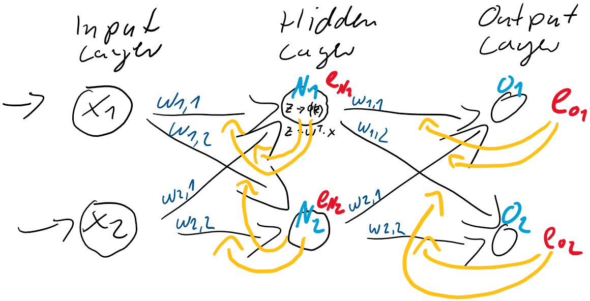
zwischen der Eingabe-Schicht I und der verborgenden Schicht N angepasst werden, entgegen dieser Fehler e_{N}.

Die Backpropagation besteht demnach aus zwei Schritten:

  1. Fehler-Berechnung durch Abgleich der Soll-Werte mit den Prädiktionen in der Ausgabeschicht und durch Fehler-Rückführung zu den Neuronen der verborgenden Schichten (Hidden-Layer)
  2. Anpassung der Gewichte entgegen des Gradientenanstiegs der Fehlerfunktion (Loss Function)

Buchempfehlungen

Die folgenden zwei Bücher haben mir sehr beim Verständnis und beim Verständlichmachen der Backpropagation in künstlichen neuronalen Netzen geholfen.

Neuronale Netze selbst programmieren: Ein verständlicher Einstieg mit Python Deep Learning. Das umfassende Handbuch: Grundlagen, aktuelle Verfahren und Algorithmen, neue Forschungsansätze (mitp Professional)

Training eines Neurons mit dem Gradientenverfahren

Dies ist Artikel 3 von 6 der Artikelserie –Einstieg in Deep Learning.

Das Training von neuronalen Netzen erfolgt nach der Forward-Propagation über zwei Schritte:

  1. Fehler-Rückführung über aller aktiver Neuronen aller Netz-Schichten, so dass jedes Neuron “seinen” Einfluss auf den Ausgabefehler kennt.
  2. Anpassung der Gewichte entgegen den Gradienten der Fehlerfunktion

Beide Schritte werden in der Regel zusammen als Backpropagation bezeichnet. Machen wir erstmal einen Schritt vor und betrachten wir, wie ein Neuron seine Gewichtsverbindungen zu seinen Vorgängern anpasst.

Gradientenabstiegsverfahren

Der Gradientenabstieg ist ein generalisierbarer Algorithmus zur Optimierung, der in vielen Verfahren des maschinellen Lernens zur Anwendung kommt, jedoch ganz besonders als sogenannte Backpropagation im Deep Learning den Erfolg der künstlichen neuronalen Netze erst möglich machen konnte.

Der Gradientenabstieg lässt sich vom Prinzip her leicht erklären: Angenommen, man stünde im Gebirge im dichten Nebel. Das Tal, und somit der Weg nach Hause, ist vom Nebel verdeckt. Wohin laufen wir? Wir können das Ziel zwar nicht sehen, tasten uns jedoch so heran, dass unser Gehirn den Gradienten (den Unterschied der Höhen beider Füße) berechnet, somit die Steigung des Bodens kennt und sich entgegen dieser Steigung unser Weg fortsetzt.

Konkret funktioniert der Gradientenabstieg so: Wir starten bei einem zufälligen Theta \theta 
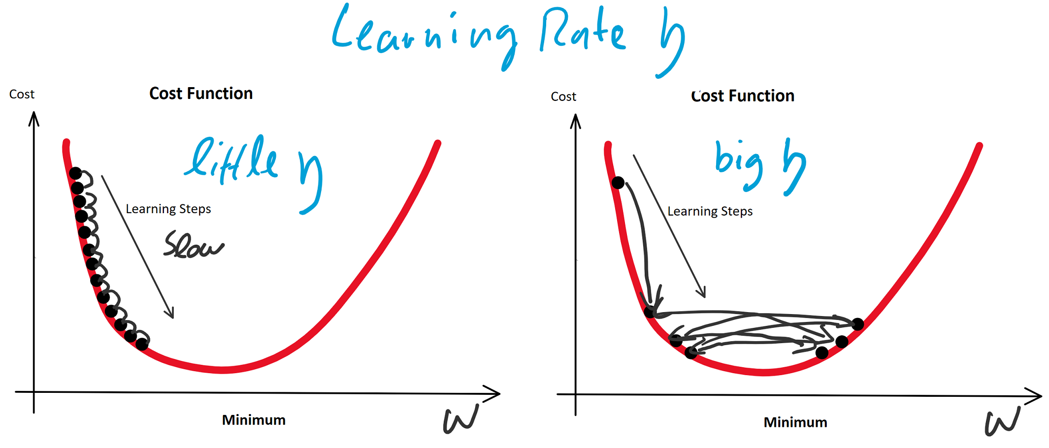
(Random Initialization). Wir berechnen die Ausgabe (Forwardpropogation) und vergleichen sie über eine Verlustfunktion (z. B. über die Funktion Mean Squared Error) mit dem tatsächlich korrekten Wert. Auf Grund der zufälligen Initialisierung haben wir eine nahe zu garantierte Falschheit der Ergebnisse und somit einen Verlust. Für die Verlustfunktion berechnen wir den Gradienten für gegebene Eingabewerte. Voraussetzung dafür ist, dass die Funktion ableitbar ist. Wir bewegen uns entgegen des Gradienten in Richtung Minimum der Verlustfunktion. Ist dieses Minimum (fast) gefunden, spricht man auch davon, dass der Lernalgorithmus konvergiert.

Das Gradientenabstiegsverfahren ist eine Möglichkeit der Gradientenverfahren, denn wollten wir maximieren, würden wir uns entlang des Gradienten bewegen, was in anderen Anwendungen sinnvoll ist.

Ob als “Cost Function” oder als “Loss Function” bezeichnet, in jedem Fall ist es eine “Error Function”, aber auf die Benennung kommen wir später zu sprechen. Jedenfalls versuchen wir die Fehlerrate zu senken! Leider sind diese Funktionen in der Praxis selten so einfach konvex (zwei Berge mit einem Tal dazwischen).


Aber Achtung: Denn befinden wir uns nur zwischen zwei Bergen, finden wir das Tal mit Sicherheit über den Gradienten. Befinden wir uns jedoch in einem richtigen Gebirge mit vielen Bergen und Tälern, gilt es, das richtige Tal zu finden. Bei der Optimierung der Gewichtungen von künstlichen neuronalen Netzen wollen wir die besten Gewichtungen finden, die uns zu den geringsten Ausgaben der Verlustfunktion führen. Wir suchen also das globale Minimum unter den vielen (lokalen) Minima.

Programmier-Beispiel in Python

Nachfolgend ein Beispiel des Gradientenverfahrens zur Berechnung einer Regression. Wir importieren numpy und matplotlib.pyplot und erzeugen uns künstliche Datenpunkte:

Nun wollen wir einen Lernalgorithmus über das Gradientenverfahren erstellen. Im Grunde haben wir hier es bereits mit einem linear aktivierten Neuron zutun:

Bei der linearen Regression, die wir durchführen wollen, nehmen wir zwei-dimensionale Daten (wobei wir die Regression prinzipiell auch mit x-Dimensionen durchführen können, dann hätte unser Neuron weitere Eingänge). Wir empfangen einen Bias (w_0
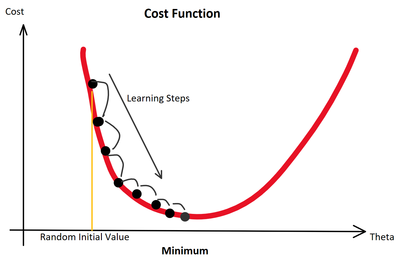
) der stets mit einer Eingangskonstante multipliziert und somit als Wert erhalten bleibt. Der Bias ist das Alpha \alpha in einer Schulmathe-tauglichen Formel wie y = \beta \cdot x + \alpha.

Beta \beta ist die Steigung, der Gradient, der Funktion.

Sowohl \alpha als auch \beta sind uns unbekannt, versuchen wir jedoch über die Betrachtung unserer Prädiktion durch Berechnung der Formel \^y = \beta \cdot x + \alpha und den darauffolgenden Abgleich mit dem tatsächlichen y herauszufinden. Anfangs behaupten wir beispielsweise einfach, sowohl \beta als auch \alpha seien 0.00. Folglich wird \^y = \beta \cdot x + \alpha ebenfalls gleich 0.00 sein und die Fehlerfunktion (Loss Function) wird maximal sein. Dies war der erste Durchlauf des Trainings, die sogenannte erste Epoche!

Die Epochen (Durchläufe) und dazugehörige Fehlergrößen. Wenn die Fehler sinken und mit weiteren Epochen nicht mehr wesentlich besser werden, heißt es, das der Lernalogorithmus konvergiert.

Als Fehlerfunktion verwenden wir bei der Regression die MSE-Funktion (Mean Squared Error):

MSE = \sum(\^y_i - y_i)^2

Um diese Funktion wird sich nun alles drehen, denn diese beschreibt den Fehler und gibt uns auch die Auskunft darüber, ob wie stark und in welche Richtung sie ansteigt, so dass wir uns entgegen der Steigung bewegen können. Wer die Regeln der Ableitung im Kopf hat, weiß, dass die Ableitung der Formel leichter wird, wenn wir sie vorher auf halbe Werte runterskalieren. Da die Proportionen dabei erhalten bleiben und uns quadrierte Fehlerwerte unserem menschlichen Verstand sowieso nicht so viel sagen (unser Gehirn denkt nunmal nicht exponential), stört das nicht:

MSE = \frac{\frac{1}{2} \cdot \sum(\^y_i - y_i)^2}{n}

MSE = \frac{\frac{1}{2} \cdot \sum(w^T \cdot x_i - y_i)^2}{n}

Wenn die Mathematik der partiellen Ableitung (Ableitung einer Funktion nach jedem Gradienten) abhanden gekommen ist, bitte nochmal folgende Regeln nachschlagen, um die nachfolgende Ableitung verstehen zu können:

  • Allgemeine partielle Ableitung
  • Kettenregel

Ableitung der MSD-Funktion nach dem einen Gewicht w 
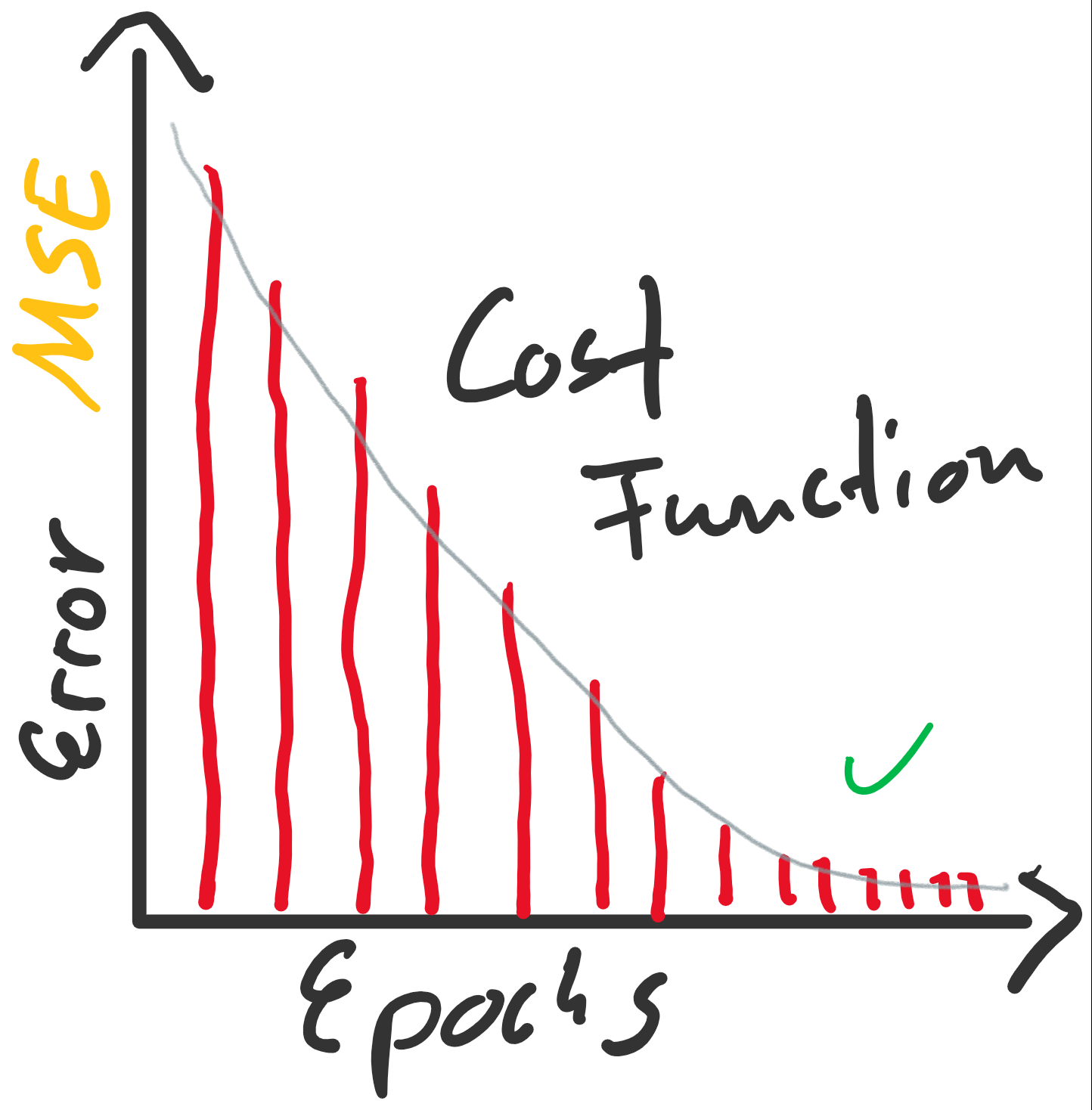
bzw. partiell nach jedem vorhandenen w_j:

\frac{\partial}{\partial w_j}MSE = \frac{\partial}{\partial w} \frac{1}{2} \cdot \sum(\^y - y_i)^2

\frac{\partial}{\partial w_j}MSE = \frac{\partial}{\partial w} \frac{1}{2} \cdot \sum(w^T \cdot x_i - y_i)^2

\frac{\partial}{\partial w_j}MSE = \frac{2}{n} \cdot \sum(w^T \cdot x_i - y_i) \cdot x_{ij}

Woher wir das x_{ij} am Ende her haben? Das ergibt sie aus der Kettenregel: Die äußere Funktion wurde abgeleitet, so wurde aus \frac{1}{2} \cdot \sum(w^T \cdot x_i - y_i)^2 dann \frac{2}{n} \cdot \sum(w^T \cdot x_i - y_i). Jedoch muss im Sinne eben dieser Kettenregel auch die innere Funktion abgeleitet werden. Da wir nach w_j ableiten, bleibt nur x_ij erhalten.

Damit können wir arbeiten! So kompliziert ist die Formel nun auch wieder nicht: \frac{2}{n} \cdot \sum(w^T \cdot x_i - y_i) \cdot x_{ij}

Mit dieser Formel können wir unsere Gewichte an den Fehler anpassen: (f\nabla ist der Gradient der Funktion!)

w_j = w_j - \nabla MSE(w_j)

Initialisieren der Gewichtungen

Die Gewichtungen \alpha und \beta müssen anfänglich mit Werten initialisiert werden. In der Regression bietet es sich an, die Gewichte anfänglich mit 0.00 zu initialisieren.

Bei vielen neuronalen Netzen, mit nicht-linearen Aktivierungsfunktionen, ist das jedoch eher ungünstig und zufällige Werte sind initial besser. Gut erprobt sind normal-verteilte Zufallswerte.

Lernrate

Nur eine Kleinigkeit haben wir bisher vergessen: Wir brauchen einen Faktor, mit dem wir anpassen. Hier wäre der Faktor 1. Das ist in der Regel viel zu groß. Dieser Faktor wird geläufig als Lernrate (Learning Rate) \eta (eta) bezeichnet:

w_j = w_j - \eta \cdot \nabla MSE(w_j)

Die Lernrate \eta ist ein Knackpunkt und der erste Parameter des Lernalgorithmus, den es anzupassen gilt, wenn das Training nicht konvergiert.

Die Lernrate \eta darf nicht zu groß klein gewählt werden, da das Training sonst zu viele Epochen benötigt. Ungeduldige erhöhen die Lernrate möglicherweise aber so sehr, dass der Lernalgorithmus im Minimum der Fehlerfunktion vorbeiläuft und diesen stets überspringt. Hier würde der Algorithmus also sozusagen konvergieren, weil nicht mehr besser werden, aber das resultierende Modell wäre weit vom Optimum entfernt.

Beginnen wir mit der Implementierung als Python-Klasse:

Die Klasse sollte so funktionieren, bevor wir sie verwenden, sollten wir die Input-Werte standardisieren:

Bei diesem Beispiel mit künstlich erzeugten Werten ist das Standardisieren bzw. das Fehlen des Standardisierens zwar nicht kritisch, aber man sollte es sich zur Gewohnheit machen. Testweise es einfach mal weglassen 🙂

Kommen wir nun zum Einsatz der Klasse, die die Regression via Gradientenabstieg absolvieren soll:

Was tut diese Instanz der Klasse LinearRegressionGD nun eigentlich?

Bildlich gesprochen, legt sie eine Gerade auf den Boden des Koordinatensystems, denn die Gewichtungen werden mit 0.00 initialisiert, y ist also gleich 0.00, egal welche Werte in x 
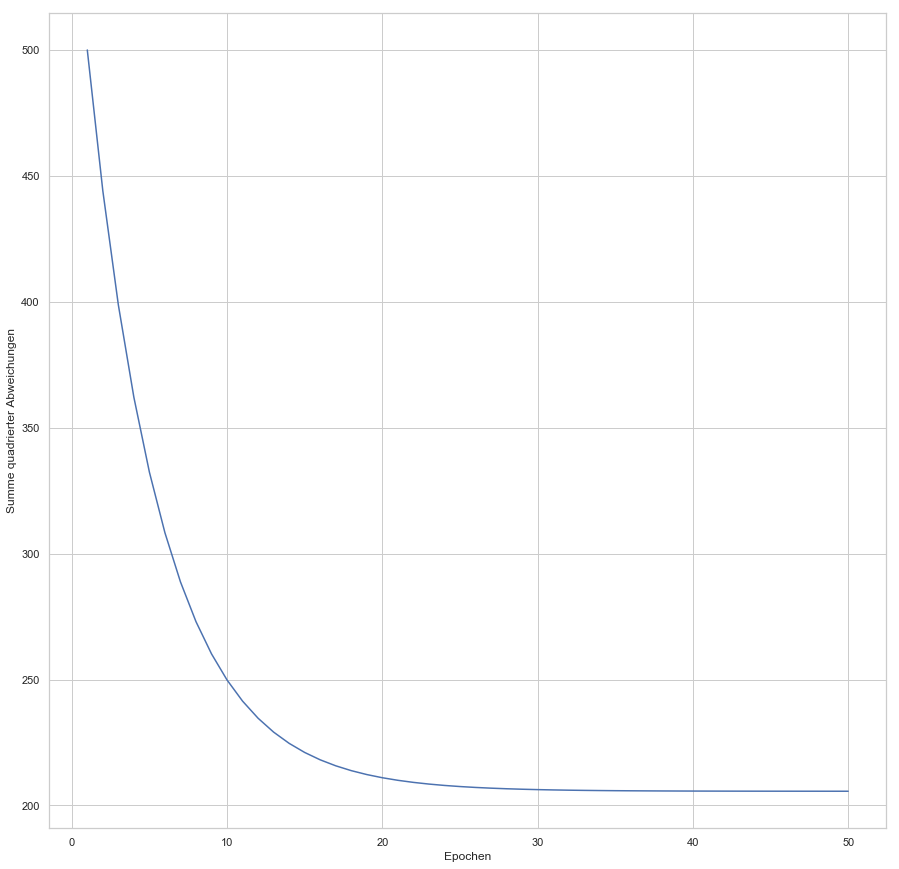
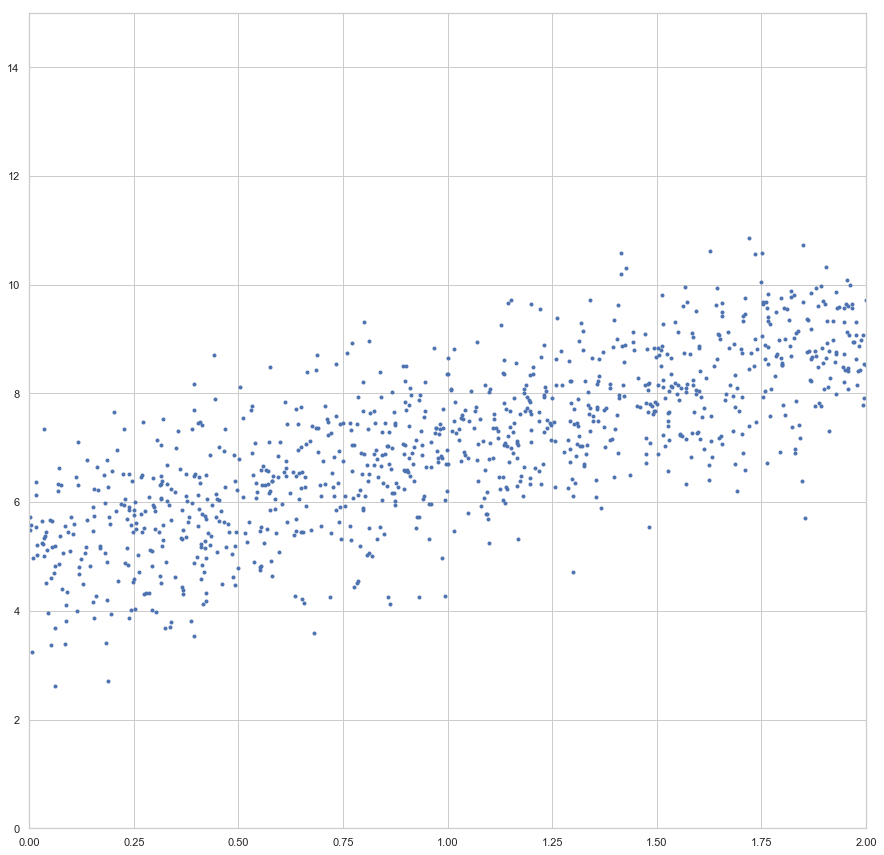
enthalten sind. Der Fehler ist dann aber sehr groß (sollte maximal sein, im Vergleich zu zukünftigen Epochen). Die Gewichte werden also angepasst, die Gerade somit besser in die Punktwolke platziert. Mit jeder Epoche wird die Gerade erneut in die Punktwolke gelegt, der Gesamtfehler (über alle
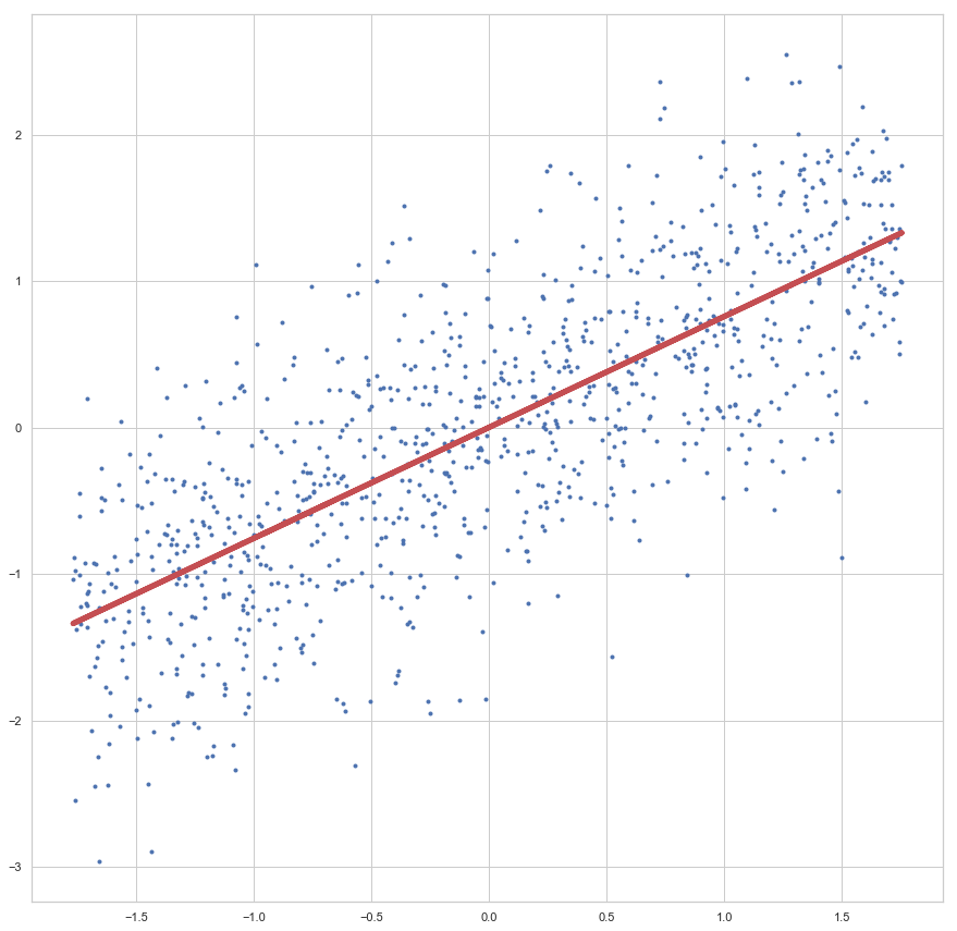
 x, da wir es hier mit dem Batch-Verfahren zutun haben) berechnet, die Werte angepasst… bis die vorgegebene Zahl an Epochen abgelaufen ist.

Schauen wir uns das Ergebnis des Trainings an:

Die Linie sieht passend aus, oder? Da wir hier nicht zu sehr in die Theorie der Regressionsanalyse abdriften möchten, lassen wir das testen und prüfen der Akkuratesse mal aus, hier möchte ich auf meinen Artikel Regressionsanalyse in Python mit Scikit-Learn verweisen.

Prüfen sollten wir hingegen mal, wie schnell der Lernalgorithmus mit der vorgegebenen Lernrate eta konvergiert:

Hier die Verlaufskurve der Cost Function:

Die Kurve zeigt uns, dass spätestens nach 40 Epochen kaum noch Verbesserung (im Sinne der Gesamtfehler-Minimierung) erreicht wird.

Wichtige Hinweise

Natürlich war das nun nur ein erster kleiner Einstieg und wer es verstanden hat, hat viel gewonnen. Denn erst dann kann man sich vorstellen, wie ein einzelnen Neuron eines künstlichen neuronalen Netzes grundsätzlich trainiert werden kann.

Folgendes sollte noch beachtet werden:

  • Lernrate \eta:
    Die Lernrate ist ein wichtiger Parameter. Wer das Programmier-Beispiel bei sich zum Laufen gebracht hat, einfach mal die Lernrate auf Werte zwischen 10.00 und 0.00000001 setzen, schauen was passiert 🙂
  • Globale Minima vs lokale Minima:
    Diese lineare zwei-dimensionale Regression ist ziemlich einfach. Neuronale Netze sind hingegen komplexer und haben nicht einfach nur eine simple konvexe Fehlerfunktion. Hier gibt es mehrere Hügel und Täler in der Fehlerfunktion und die Gefahr ist groß, in einem lokalen, nicht aber in einem globalen Minimum zu landen.
  • Stochastisches Gradientenverfahren:
    Wir haben hier das sogenannte Batch-Verfahren verwendet. Dieses ist grundsätzlich besser als die stochastische Methode. Denn beim Batch verwenden wir den gesamten Stapel an x-Werten für die Fehlerbestimmung. Allerdings ist dies bei großen Daten zu rechen- und speicherintensiv. Dann werden kleinere Unter-Stapel (Sub-Batches) zufällig aus den x-Werten ausgewählt, der Fehler daraus bestimmt (was nicht ganz so akkurat ist, wie als würden wir den Fehler über alle x berechnen) und der Gradient bestimmt. Dies ist schon Rechen- und Speicherkapazität, erfordert aber meistens mehr Epochen.

Buchempfehlung

Die folgenden zwei Bücher haben mir bei der Erstellung dieses Beispiels geholfen und kann ich als hilfreiche und deutlich weiterführende Lektüre empfehlen:


Machine Learning mit Python und Scikit-Learn und TensorFlow: Das umfassende Praxis-Handbuch für Data Science, Predictive Analytics und Deep Learning (mitp Professional) Hands-On Machine Learning with Scikit-Learn and TensorFlow: Concepts, Tools, and Techniques for Building Intelligent Systems


Künstliche Intelligenz und Vorurteil

Kaum ein anderes technologisches Thema heutzutage wird hinsichtlich gesellschaftlicher Auswirkungen so kontrovers diskutiert wie das der Künstlichen Intelligenz (KI). Während das Wörtchen „KI“ bei den einen Zukunftsvisionen hervorruft, in welchen technologischer Fortschritt menschliche Probleme wie Hunger, Krankheit und Klimawandel reduziert hat, zeichnen andere düstere Bilder von Orwell‘schen Überwachungsstaaten und technologischen Apokalypsen.

Starke, schwache KI

Es ist die Unschärfe des Begriffes „KI“, welcher eine derart große Bandbreite an Zukunftsszenarien ermöglicht. Für diejenigen, welche sich an solch spekulativen Debatten beteiligen, beutet KI „starke KI“ – eine künstliche Intelligenz, deren intellektuellen Fähigkeiten die eines Menschen erreichen oder gar übertreffen. Und so spannend die Diskussion über starke KI auch ist – sie ist reine Spekulation. Heute existierende KI ist weit, sehr weit von starker KI entfernt. Worüber wir heutzutage verfügen ist die sogenannte „schwache KI“ – Algorithmen, die spezifische Anwendungsprobleme (z.B. Bilderkennung, Spracherkennung, Übersetzung, Go spielen) lösen können. Und das mitunter sehr viel besser als Menschen.

Wo heutzutage „KI“ draufsteht, sind innen überwiegend Algorithmen aus dem Bereich des maschinellen Lernens (allen voran Deep Learning) am Werk. Diese Algorithmen können selbständig die Vorgehensweise erlernen, die zum Beispiel nötig ist, um einen gegebenen Input (z.B. ein Bild) auf einen gegebenen Output (z.B. eine Kategorie, welche den Bildinhalt beschreibt) abzubilden. Aber selbst diese „schwache KI“ birgt beträchtliches Potential – denken wir an mögliche Verbesserungen z.B. im Bereich der Medizin, Logistik, Verkehrssicherheit oder Energie- und Ressourcennutzung! Angesichts der Chancen, heutige Prozesse und Anwendungen zu verbessern, haben wir allen Grund, dem Einsatz von KI aufgeschlossen gegenüber zu stehen. Vorausgesetzt natürlich, dass KI verantwortungsvoll, „ethisch“ und sicher eingesetzt wird.

KI auf Abwegen

Ethische Herausforderungen von KI ergeben sich dabei zum einen durch die Zielsetzung. Wie ein Hammer für den Nagel an der Wand oder für den Hinterkopf eines Gegners verwendet werden kann, kann auch KI für böse Ziele missbraucht werden. Nur, dass KI im Zweifel deutlich größeren Schaden anrichten kann als ein einfacher Hammer. Und so sollten wir angesichts der Risiken dringend international diskutieren, wie wir uns hinsichtlich militärischer Anwendungen von KI verhalten wollen.

Zum anderen dringen besonders aus den USA, in denen KI Algorithmen schon heute in deutlich größerem Ausmaß eingesetzt werden als in Deutschland, immer wieder beunruhigende Nachrichten über voreingenommene KI Algorithmen. Zum ersten fand eine Studie kürzlich heraus, dass kommerziell erhältliche Gesichtserkennungsalgorithmen für Frauen bzw. dunkelhäutige Menschen schlechter funktionieren als für Männer bzw. hellhäutige Menschen. Mit der unschönen Konsequenz, dass es z.B. bei einem Abgleich mit Verbrecherfotos bei Menschen mit dunkler Hautfarbe deutlich häufiger zu falschen Übereinstimmungen kommen kann als bei Menschen heller Hautfarbe. Zum zweiten wurde vor kurzem bekannt, dass eine experimentell von einem großen Technologiekonzern zur Bewertung von Bewerbungen verwendete KI von Frauen stammende Bewerbungen systematisch schlechter bewertete als von Männern stammende Bewerbungen.

Wie KI zu Vorurteilen kommt

Um die Ursachen für vorurteilsbehaftete KI besser zu verstehen, lohnt es sich, einen Blick hinter die Kulissen zu werfen. Denn wie jede Technologie existiert auch KI nicht im luftleeren Raum. Dies lässt sich leicht anhand der Faktoren verdeutlichen, welche zum Erfolg heutiger KI beigetragen haben: bessere Hardware, cleverere Algorithmen und größere Datenmengen. Und gerade diese Daten sind es, durch welche Vorurteile in KI Einzug halten können.

Die Vorstellung von „neutralen Daten“ ist nämlich eine Wunschvorstellung. Im besten Fall spiegeln Daten die Welt wider, in der wir leben.       Eine Welt zum Beispiel, in der in Technologiekonzernen typischerweise deutlich mehr Männer beschäftigt sind als Frauen – was eine auf dem Personalbestand eines Technologiekonzerns trainierte KI dazu veranlassen kann, zu „schlussfolgern“, dass männliche Bewerber im Auswahlverfahren zu bevorzugen sind. Oder eine Welt, in der Länder bzw. gesellschaftliche Schichten innerhalb eines Landes unterschiedlichen Zugang zu modernen Technologien oder auch Bildung haben. Eine Ungleichheit, die sich als Dominanz westlicher Industrienationen in der geografischen Zusammensetzung von zum Training von KI-Algorithmen verwendeter Datensätze auswirken kann. Eine Dominanz, die wiederum zur Folge haben kann, dass derart trainierte KI-Algorithmen besonders gut für Menschen aus westlichen Industrienationen funktionieren. Ganz zu schweigen von der Voreingenommenheit der menschlichen Wahrnehmung, welche die Zusammensetzung von Daten beeinflusst – denken wir an das begrenzte Spektrum der Bilder, welche uns zuerst zu dem Begriff „Genie“ in den Sinn kommen.

Aber nicht nur die verwendeten Trainingsdaten, sondern auch bei der Entwicklung von KI getroffenen Design-Entscheidungen können negative Auswirkungen haben. Wenn bei einem nicht perfekt funktionierenden Bilderkennungsalgorithmus potentiell abwertende Kategorien zur Klassifikation zur Verfügung stehen, kann dies dazu führen, dass – wie in der Vergangenheit geschehen – dunkelhäutige Menschen als Gorillas klassifiziert werden. Wenn bei der Evaluation eines z.B. für die Gesichtserkennung eingesetzten KI-Algorithmus nur die Genauigkeit über alle Bevölkerungsgruppen hinweg berücksichtigt wird, können Ungleichheiten in der Genauigkeit nicht entdeckt werden, was zu Problemen bei der Anwendung führen kann. Denn Nutzer von KI-Algorithmen vermuten zumeist, dass die Algorithmen für alle denkbaren Anwendungszwecke geeignet sind.

Werte statt Wegsehen

Entgegen der verbreiteten Auffassung sind KI Algorithmen also nicht notwendigerweise vorurteilsfrei – sie können menschliche Voreingenommenheit bzw. gesellschaftliche Ungleichheit widerspiegeln. Da Algorithmen anders und in anderem Maß als Menschen eingesetzt werden, kann das bei blauäugiger Verwendung dazu führen, dass bestehende Ungleichheiten nicht nur bestärkt, sondern sogar vergrößert werden. Richtig angewendet können Algorithmen jedoch helfen, implizite und explizite Vorurteile menschlicher Entscheider zu mindern. Denn wie wir durch viele Studien wissen, ist die Liste der kognitiven Verzerrungen, die wir Menschen aufweisen, lang.

Es ist für den verantwortlichen Einsatz von KI in einem sensiblen Kontext somit essenziell, zu wissen, welche „ethischen“ Kriterien KI für den konkreten Anwendungsfall erfüllen muss. So kann sichergestellt werden, dass die KI den Anforderungen entspricht, bevor sie angewendet wird – oder aber, dass sie solange nicht angewendet wird, wie sie den Anforderungen nicht entspricht. Und mittels Transparenz, Überwachung und Feedback-Möglichkeiten lässt sich vermeiden, dass ein selbst-verbessernder KI-Algorithmus im Laufe der Zeit das ihm gesteckte Ziel verfehlt.

Für viele Anwendungsfälle sind derartige ethische Fragen jedoch vernachlässigbar, denken wir zum Beispiel an die Vorhersage von Maschinenausfällen oder die Extraktion strukturierter Daten aus unstrukturierten Dokumenten. Aber es ist nichtsdestotrotz gut und wichtig, Ethik und KI zusammen zu denken. Denn dies ermöglicht es uns, sicherzustellen, dass wir KI auf die bestmögliche Weise einsetzen. Denn das enorme Potential von KI gibt uns die Chance, den Status quo nachhaltig positiv zu verändern – technologisch wie ethisch.