Einführung in die Welt der Autoencoder

An wen ist der Artikel gerichtet?

In diesem Artikel wollen wir uns näher mit dem neuronalen Netz namens Autoencoder beschäftigen und wollen einen Einblick in die Grundprinzipien bekommen, die wir dann mit einem vereinfachten Programmierbeispiel festigen. Kenntnisse in Python, Tensorflow und neuronalen Netzen sind dabei sehr hilfreich.

Funktionsweise des Autoencoders

Ein Autoencoder ist ein neuronales Netz, welches versucht die Eingangsinformationen zu komprimieren und mit den reduzierten Informationen im Ausgang wieder korrekt nachzubilden.

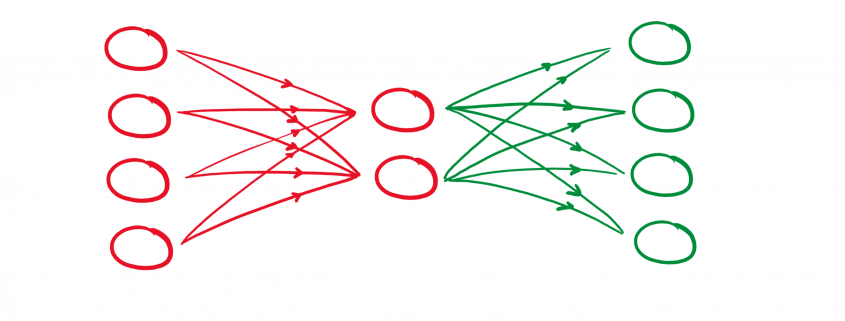
Die Komprimierung und die Rekonstruktion der Eingangsinformationen laufen im Autoencoder nacheinander ab, weshalb wir das neuronale Netz auch in zwei Abschnitten betrachten können.


Der Encoder

Der Encoder oder auch Kodierer hat die Aufgabe, die Dimensionen der Eingangsinformationen zu reduzieren, man spricht auch von Dimensionsreduktion. Durch diese Reduktion werden die Informationen komprimiert und es werden nur die wichtigsten bzw. der Durchschnitt der Informationen weitergeleitet. Diese Methode hat wie viele andere Arten der Komprimierung auch einen Verlust.

In einem neuronalen Netz wird dies durch versteckte Schichten realisiert. Durch die Reduzierung von Knotenpunkten in den kommenden versteckten Schichten werden die Kodierung bewerkstelligt.

Der Decoder

Nachdem das Eingangssignal kodiert ist, kommt der Decoder bzw. Dekodierer zum Einsatz. Er hat die Aufgabe mit den komprimierten Informationen die ursprünglichen Daten zu rekonstruieren. Durch Fehlerrückführung werden die Gewichte des Netzes angepasst.

Ein bisschen Mathematik

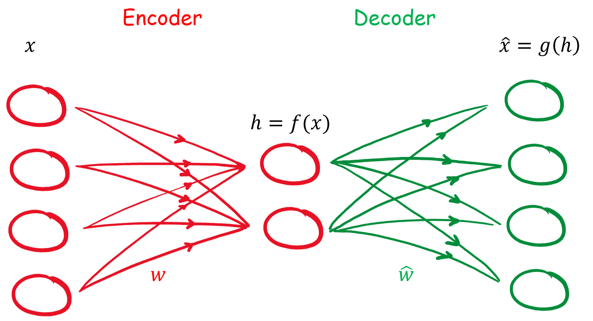
Das Hauptziel des Autoencoders ist, dass das Ausgangssignal dem Eingangssignal gleicht, was bedeutet, dass wir eine Loss Funktion haben, die L(x , y) entspricht.

L(x, \hat{x})

Unser Eingang soll mit x gekennzeichnet werden. Unsere versteckte Schicht soll h sein. Damit hat unser Encoder folgenden Zusammenhang h = f(x).

Die Rekonstruktion im Decoder kann mit r = g(h) beschrieben werden. Bei unserem einfachen Autoencoder handelt es sich um ein Feed-Forward Netz ohne rückkoppelten Anteil und wird durch Backpropagation oder zu deutsch Fehlerrückführung optimiert.

Formelzeichen Bedeutung
\mathbf{x}, \hat{\mathbf{x}} Eingangs-, Ausgangssignal
\mathbf{W}, \hat{\mathbf{W}} Gewichte für En- und Decoder
\mathbf{B}, \hat{\mathbf{B}} Bias für En- und Decoder
\sigma, \hat{\sigma} Aktivierungsfunktion für En- und Decoder
L Verlustfunktion

Unsere versteckte Schicht soll mit \latex h gekennzeichnet werden. Damit besteht der Zusammenhang:

(1)   \begin{align*} \mathbf{h} &= f(\mathbf{x}) = \sigma(\mathbf{W}\mathbf{x} + \mathbf{B}) \\ \hat{\mathbf{x}} &= g(\mathbf{h}) = \hat{\sigma}(\hat{\mathbf{W}} \mathbf{h} + \hat{\mathbf{B}}) \\ \hat{\mathbf{x}} &= \hat{\sigma} \{ \hat{\mathbf{W}} \left[\sigma ( \mathbf{W}\mathbf{x} + \mathbf{B} )\right]  + \hat{\mathbf{B}} \}\\ \end{align*}

Für eine Optimierung mit der mittleren quadratischen Abweichung (MSE) könnte die Verlustfunktion wie folgt aussehen:

(2)   \begin{align*} L(\mathbf{x}, \hat{\mathbf{x}}) &= \mathbf{MSE}(\mathbf{x}, \hat{\mathbf{x}}) = \|  \mathbf{x} - \hat{\mathbf{x}} \| ^2 &=  \| \mathbf{x} - \hat{\sigma} \{ \hat{\mathbf{W}} \left[\sigma ( \mathbf{W}\mathbf{x} + \mathbf{B} )\right]  + \hat{\mathbf{B}} \} \| ^2 \end{align*}


Wir haben die Theorie und Mathematik eines Autoencoder in seiner Ursprungsform kennengelernt und wollen jetzt diese in einem (sehr) einfachen Beispiel anwenden, um zu schauen, ob der Autoencoder so funktioniert wie die Theorie es besagt.

Dazu nehmen wir einen One Hot (1 aus n) kodierten Datensatz, welcher die Zahlen von 0 bis 3 entspricht.

    \begin{align*} [1, 0, 0, 0] \ \widehat{=}  \ 0 \\ [0, 1, 0, 0] \ \widehat{=}  \ 1 \\ [0, 0, 1, 0] \ \widehat{=}  \ 2 \\ [0, 0, 0, 1] \ \widehat{=} \  3\\ \end{align*}

Diesen Datensatz könnte wie folgt kodiert werden:

    \begin{align*} [1, 0, 0, 0] \ \widehat{=}  \ 0 \ \widehat{=}  \ [0, 0] \\ [0, 1, 0, 0] \ \widehat{=}  \ 1 \ \widehat{=}  \  [0, 1] \\ [0, 0, 1, 0] \ \widehat{=}  \ 2 \ \widehat{=}  \ [1, 0] \\ [0, 0, 0, 1] \ \widehat{=} \  3 \ \widehat{=}  \ [1, 1] \\ \end{align*}

Damit hätten wir eine Dimensionsreduktion von vier auf zwei Merkmalen vorgenommen und genau diesen Vorgang wollen wir bei unserem Beispiel erreichen.

Programmierung eines einfachen Autoencoders


Typische Einsatzgebiete des Autoencoders sind neben der Dimensionsreduktion auch Bildaufarbeitung (z.B. Komprimierung, Entrauschen), Anomalie-Erkennung, Sequenz-to-Sequenz Analysen, etc.

Ausblick

Wir haben mit einem einfachen Beispiel die Funktionsweise des Autoencoders festigen können. Im nächsten Schritt wollen wir anhand realer Datensätze tiefer in gehen. Auch soll in kommenden Artikeln Variationen vom Autoencoder in verschiedenen Einsatzgebieten gezeigt werden.

Article series: 5 Clean Coding Tips – 2. Name Variables in a Meaningful Way

This is the second of the article series “5 tips for clean coding” to follow as soon as you’ve made the first steps into your coding career, in this article series. Read the introduction here, to find out why it is important to write clean code if you missed it.

When it comes to naming variables, there are a few official rules in the PEP8 style guide. A variable must start with an underscore or a letter and can be followed by a number of underscores or letters or digits. They cannot be reserved words: True, False, or, not, lambda etc. The preferred naming style is lowercase or lowercase_with_underscore. This all refers to variable names on a visual level. However, for readability purposes, the semantic level is as important, or maybe even more so. If it was for python, the variables could be named like this:

It wouldn’t make the slightest difference. But again, the code is not only for the interpreter to be read. It is for humans. Other people might need to look at your code to understand what you did, to be able to continue the work that you have already started. In any case, they need to be able to decipher what hides behind the variable names, that you’ve given the objects in your code. They will need to remember what they meant as they reappear in the code. And it might not be easy for them.

Remembering names is not an easy thing to do in all life situations. Let’s consider the following situation. You go to a party, there is a bunch of new people that you meet for the first time. They all have names and you try very hard to remember them all. Imagine how much easier would it be if you could call the new girl who came with John as the_girl_who_came_with_John. How much easier would it be to gossip to your friends about her? ‘Camilla is on the 5th glass of wine tonight, isn’t she?!.’ ‘Who are you talking about???’ Your friends might ask. ‘The_Girl_who_came_with_John.’ And they will all know. ‘It was nice to meet you girl_who_came_with_john, see you around.’ The good thing is that variables are not really like people. You can be a bit rude to them, they will not mind. You don’t have to force yourself or anyone else to remember an arbitrary name of a variable, that accidentally came to your mind in the moment of creation. Let your colleagues figure out what is what by a meaningful, straightforward description of it.

There is an important tradeoff to be aware of here. The lines of code should not exceed a certain length (79 characters, according to the PEP 8), therefore, it is recommended that you keep your names as short as possible. It is worth to give it a bit of thought about how you can name your variable in the most descriptive way, keeping it as short as possible. Keep in mind, that
the_blond_girl_in_a_dark_blue_dress_who_came_with_John_to_this_party might not be the best choice.

There are a few additional pieces of advice when it comes to naming your variables. First, try to always use pronounceable names. If you’ve ever been to an international party, you will know how much harder to remember is something that you cannot even repeat. Second, you probably have been taught over and over again that whenever you create a loop, you use i and j to denote the iterators.

It is probably engraved deep into the folds in your brain to write for i in…. You need to try and scrape it out of your cortex. Think about what the i stands for, what it really does and name it accordingly. Is i maybe the row_index? Is it a list_element?

Additionally, think about when to use a noun and where a verb. Variables usually are things and functions usually do things. So, it might be better to name functions with verb expressions, for example: get_id() or raise_to_power().

Moreover, it is a good practice to name constant numbers in the code. First, because when you name them you explain the meaning of the number. Second, because maybe one day you will have to change that number. If it appears multiple times in your code, you will avoid searching and changing it in every place. PEP 8 states that the constants should be named with UPPER_CASE_NAME. It is also quite common practice to explain the meaning of the constants with an inline comment at the end of the line, where the number appears. However, this approach will increase the line length and will require repeating the comment if the number appears more than one time in the code.

How Important is Customer Lifetime Value?

This is the third article of article series Getting started with the top eCommerce use cases.

Customer Lifetime Value

Many researches have shown that cost for acquiring a new customer is higher than the cost of retention of an existing customer which makes Customer Lifetime Value (CLV or LTV) one of the most important KPI’s. Marketing is about building a relationship with your customer and quality service matters a lot when it comes to customer retention. CLV is a metric which determines the total amount of money a customer is expected to spend in your business.

CLV allows marketing department of the company to understand how much money a customer is going  to spend over their  life cycle which helps them to determine on how much the company should spend to acquire each customer. Using CLV a company can better understand their customer and come up with different strategies either to retain their existing customers by sending them personalized email, discount voucher, provide them with better customer service etc. This will help a company to narrow their focus on acquiring similar customers by applying customer segmentation or look alike modeling.

One of the main focus of every company is Growth in this competitive eCommerce market today and price is not the only factor when a customer makes a decision. CLV is a metric which revolves around a customer and helps to retain valuable customers, increase revenue from less valuable customers and improve overall customer experience. Don’t look at CLV as just one metric but the journey to calculate this metric involves answering some really important questions which can be crucial for the business. Metrics and questions like:

  1. Number of sales
  2. Average number of times a customer buys
  3. Full Customer journey
  4. How many marketing channels were involved in one purchase?
  5. When the purchase was made?
  6. Customer retention rate
  7. Marketing cost
  8. Cost of acquiring a new customer

and so on are somehow associated with the calculation of CLV and exploring these questions can be quite insightful. Lately, a lot of companies have started to use this metric and shift their focuses in order to make more profit. Amazon is the perfect example for this, in 2013, a study by Consumers Intelligence Research Partners found out that prime members spends more than a non-prime member. So Amazon started focusing on Prime members to increase their profit over the past few years. The whole article can be found here.

How to calculate CLV?

There are several methods to calculate CLV and few of them are listed below.

Method 1: By calculating average revenue per customer


Figure 1: Using average revenue per customer


Let’s suppose three customers brought 745€ as profit to a company over a period of 2 months then:

CLV (2 months) = Total Profit over a period of time / Number of Customers over a period of time

CLV (2 months) = 745 / 3 = 248 €

Now the company can use this to calculate CLV for an year however, this is a naive approach and works only if the preferences of the customer are same for the same period of time. So let’s explore other approaches.

Method 2

This method requires to first calculate KPI’s like retention rate and discount rate.


CLV = Gross margin per lifespan ( Retention rate per month / 1 + Discount rate – Retention rate per month)

Where

Retention rate = Customer at the end of the month – Customer during the month / Customer at the beginning of the month ) * 100

Method 3

This method will allow us to look at other metrics also and can be calculated in following steps:

  1. Calculate average number of transactions per month (T)
  2. Calculate average order value (OV)
  3. Calculate average gross margin (GM)
  4. Calculate customer lifespan in months (ALS)

After calculating these metrics CLV can be calculated as:


CLV = T*OV*GM*ALS / No. of Clients for the period

where

Transactions (T) = Total transactions / Period

Average order value (OV) = Total revenue / Total orders

Gross margin (GM) = (Total revenue – Cost of sales/ Total revenue) * 100 [but how you calculate cost of sales is debatable]

Customer lifespan in months (ALS) = 1 / Churn Rate %


CLV can be calculated using any of the above mentioned methods depending upon how robust your company wants the analysis to be. Some companies are also using Machine learning models to predict CLV, maybe not directly but they use ML models to predict customer churn rate, retention rate and other marketing KPI’s. Some companies take advantage of all the methods by taking an average at the end.

Matrix search: Finding the blocks of neighboring fields in a matrix with Python

Task

In this article we will look at a solution in python to the following grid search task:

Find the biggest block of adjoining elements of the same kind and into how many blocks the matrix is divided. As adjoining blocks, we will consider field touching by the sides and not the corners.

Input data

For the ease of the explanation, we will be looking at a simple 3×4 matrix with elements of three different kinds, 0, 1 and 2 (see above). To test the code, we will simulate data to achieve different matrix sizes and a varied number of element types. It will also allow testing edge cases like, where all elements are the same or all elements are different.

To simulate some test data for later, we can use the numpy randint() method:

The code

How the code works

In summary, the algorithm loops through all fields of the matrix looking for unseen fields that will serve as a starting point for a local exploration of each block of color – the find_blocks() function. The local exploration is done by looking at the neighboring fields and if they are within the same kind, moving to them to explore further fields – the explore_block() function. The fields that have already been seen and counted are stored in the visited list.

find_blocks() function:

  1. Finds a starting point of a new block
  2. Runs a the explore_block() function for local exploration of the block
  3. Appends the size of the explored block
  4. Updates the list of visited points
  5. Returns the result, once all fields of the matrix have been visited.

explore_block() function:

  1. Takes the coordinates of the starting field for a new block and the list of visited points
  2. Creates the queue set with the starting point
  3. Sets the size of the current block (field_count) to 1
  4. Starts a while loop that is executed for as long as the queue is not empty
    1. Takes an element of the queue and uses its coordinates as the current location for further exploration
    2. Adds the current field to the visited list
    3. Explores the neighboring fields and if they belong to the same block, they are added to the queue
    4. The fields are taken off the queue for further exploration one by one until the queue is empty
  5. Returns the field_count of the explored block and the updated list of visited fields

Execute the function

The returned result is biggest block: 4, number of blocks: 4.

Run the test matrices:

Visualization

The matrices for the article were visualized with the seaborn heatmap() method.

Article series: 5 Clean Coding Tips – 1. Be Consistent

This is the first of the article series “5 tips for clean coding” to follow as soon as you’ve made the first steps into your coding career, in this article series. Read the introduction here, to find out why it is important to write clean code if you missed it.

Consistency is THE rule to follow if you want to make your code clean and increase readability. Not to make it sound desperate, but honestly, whatever you decide to do when it comes to the coding style, just be consistent. Whether you agree with any standards, formatting styles or don’t even know them, just be consistent. Don’t ever allow inconsistency to sneak into your script or your project. This will only bring confusion, disorientation, chaos and general misery.

The rules for how exactly keep your code clean and organized visually might differ slightly depending on the situation you find yourself in. The PEP 8 rules can be ambiguous in some places and leave room for interpretation. For example, the question, whether you use single or double quotes to denote a string, is open. It is possible, that your work environment already has a standard and you just need to comply with that. No room to show off your highly unique take on it, sorry. However, if you are working on your own and there is no one to roll their eyes looking at your messed-up code, you need to decide for yourself. Once you do, again, be consistent at the level of the script, project, your work in general. Otherwise, it will look messy, patchworky and simply unprofessional.

People famously are quick to ascribe intentionality, even to thermostats[i]. They will assume that the details of how you wrote your code are intentional. They will try to figure out why you are doing one thing in some places and a different thing in other places. If those differences came from you being careless and have no meaning behind them, the reader of your code will waste a lot of time trying to figure it out and end up frustrated. Remember the first few snippets of python code you have ever seen? Maybe you saw some code with double quotes and some with single quotes. You were green, knew nothing and quite possibly thought that they both have different meanings and you spent time trying to figure out why on earth in some places there is a single quote and in other double-quotes.

If those altruistic arguments do not really convince you, let’s see how consistency can serve to your own benefit. First, that outsider, who is looking at your code and is trying very hard to figure out what on Earth is going on, might be you. It might sound crazy, and it is, indeed, quite sad, but most likely, after 6 months of not looking at your code you will no longer remember what you did there if it is not documented well. Documenting in a homogenous way can take some time and some effort. Nevertheless, in general, code gets read many times after it has been written. When in doubt, sacrifice some of your writing time to increase readability and minimize the reading time later. It will pay off in the long run.

Having a set of rules at your disposal can make your work faster. You will avoid arguing with yourself about which option is the best one: mean_income, income_mean or income_avg. You can avoid making loads of small decisions as you write your code by making a set of global rules. In that way, you can allocate your energy and resources into solving the real problem. Not the how-do-I-format-this? one.

It is not necessary that you make all those grand decisions right now. You also don’t have to make them for life, it’s ok to change your mind eventually, so don’t feel overwhelmed. But once you’ve learned this and that, spent a little time coding, have a good long look at your sprouting habits and decide what you are going to do about splitting those lines and stick to it!

References:

[i] https://en.wikipedia.org/wiki/Intentional_stance

Article series: 5 Clean Coding Tips

This series of articles will cover 5 clean coding tips to follow as soon as you’ve made the first steps into your coding career, with the example of python.

At the beginning of your adventure with coding, you might find that getting your code to compile without any errors and give you the output that you expect is hard enough. Conforming to any standards and style guides is at the very bottom of your concerns. You might be at the beginning of your career or you might have a lot of domain experience but not that much in coding. Or maybe until now you worked mostly on your own and never had to make your code available for others to work with it. In any case, it is worth acknowledging how crucial it is to write your code in a concise, readable and understandable way, and how much benefits it will eventually bring you.

The first thing to realize is that the whole clean coding concept has been developed for people, your fellow travelers, not for the computers. The compiler doesn’t care how you name your variables, how you split your lines or if everything is aligned in a pretty way. You could even write your code as a one gigantic, few-meters-long line, giving the interpreter just a signal – a semicolon, that the line should be split, and it will execute it perfectly.

However, it is likely that, the deeper you are into your career, the more people will have to read, understand and modify the code that you wrote. You will write code to communicate certain ideas and solutions with other people. Therefore, you need to be sure, that what you want to communicate is understandable, easy and quick to read. The coding best practice is to always code in a clean way, treating the code itself and not just the output as the result of your work.

There usually are fixed rules and standards regarding code readability. For python, it is the PEP 8[i]. Some companies elaborate on those standards where the PEP 8 is a bit vague or leaves room for interpretation. The exact formatting styles might differ at Facebook, Google[ii] or at the company you happen to work for. But before you get lost in the art of a perfect line splitting, brackets alignment technique, or the hopeless tabs or spaces battle, have a look at the 5 tips in the upcoming articles in this series. They are universal and might help you make your code, less of a chaotic mess and more of blissful delight.

List of articles in this series:

  1. Be consistent
  2. Name variables in a meaningful way
  3. Take advantage of the formatting tools
  4. Stop commenting the obvious
  5. Put yourself in somebody else’s shoes
References:

[i] https://www.python.org/dev/peps/pep-0008/
[ii] http://google.github.io/styleguide/pyguide.html

Introduction to Recommendation Engines

This is the second article of article series Getting started with the top eCommerce use cases. If you are interested in reading the first article you can find it here.

What are Recommendation Engines?

Recommendation engines are the automated systems which helps select out similar things whenever a user selects something online. Be it Netflix, Amazon, Spotify, Facebook or YouTube etc. All of these companies are now using some sort of recommendation engine to improve their user experience. A recommendation engine not only helps to predict if a user prefers an item or not but also helps to increase sales, ,helps to understand customer behavior, increase number of registered users and helps a user to do better time management. For instance Netflix will suggest what movie you would want to watch or Amazon will suggest what kind of other products you might want to buy. All the mentioned platforms operates using the same basic algorithm in the background and in this article we are going to discuss the idea behind it.

What are the techniques?

There are two fundamental algorithms that comes into play when there’s a need to generate recommendations. In next section these techniques are discussed in detail.

Content-Based Filtering

The idea behind content based filtering is to analyse a set of features which will provide a similarity between items themselves i.e. between two movies, two products or two songs etc. These set of features once compared gives a similarity score at the end which can be used as a reference for the recommendations.

There are several steps involved to get to this similarity score and the first step is to construct a profile for each item by representing some of the important features of that item. In other terms, this steps requires to define a set of characteristics that are discovered easily. For instance, consider that there’s an article which a user has already read and once you know that this user likes this article you may want to show him recommendations of similar articles. Now, using content based filtering technique you could find the similar articles. The easiest way to do that is to set some features for this article like publisher, genre, author etc. Based on these features similar articles can be recommended to the user (as illustrated in Figure 1). There are three main similarity measures one could use to find the similar articles mentioned below.


Figure 1: Content-Based Filtering


Minkowski distance

Minkowski distance between two variables can be calculated as:

(x,y)= (\sum_{i=1}^{n}{|X_{i} - Y_{i}|^{p}})^{1/p}


Cosine Similarity

Cosine similarity between two variables can be calculated as :

  \mbox{Cosine Similarity} = \frac{\sum_{i=1}^{n}{x_{i} y_{i}}} {\sqrt{\sum_{i=1}^{n}{x_{i}^{2}}} \sqrt{\sum_{i=1}^{n}{y_{i}^{2}}}} \


Jaccard Similarity


  J(X,Y) = |X ∩ Y| / |X ∪ Y|


These measures can be used to create a matrix which will give you the similarity between each movie and then a function can be defined to return the top 10 similar articles.


Collaborative filtering

This filtering method focuses on finding how similar two users or two products are by analyzing user behavior or preferences rather than focusing on the content of the items. For instance consider that there are three users A,B and C.  We want to recommend some movies to user A, our first approach would be to find similar users and compare which movies user A has not yet watched and recommend those movies to user A.  This approach where we try to find similar users is called as User-User Collaborative Filtering.  

The other approach that could be used here is when you try to find similar movies based on the ratings given by others, this type is called as Item-Item Collaborative Filtering. The research shows that item-item collaborative filtering works better than user-user collaborative filtering as user behavior is really dynamic and changes over time. Also, there are a lot more users and increasing everyday but on the other side item characteristics remains the same. To calculate the similarities we can use Cosine distance.


Figure 2: Collaborative Filtering


Recently some companies have started to take advantage of both content based and collaborative filtering techniques to make a hybrid recommendation engine. The results from both models are combined into one hybrid model which provides more accurate recommendations. Five steps are involved to make a recommendation engine work which are collection of data, storing of data, analyzing the data, filtering the data and providing recommendations. There are a lot of attributes that are involved in order to collect user data including browsing history, page views, search logs, order history, marketing channel touch points etc. which requires a strong data architecture.  The collection of data is pretty straightforward but it can be overwhelming to analyze this amount of data. Storing this data could get tricky on the other hand as you need a scalable database for this kind of data. With the rise of graph databases this area is also improving for many use cases including recommendation engines. Graph databases like Neo4j can also help to analyze and find similar users and relationship among them. Analyzing the data can be carried in different ways, depending on how strong and scalable your architecture you can run real time, batch or near real time analysis. The fourth step involves the filtering of the data and here you can use any of the above mentioned approach to find similarities to finally provide the recommendations.

Having a good recommendation engine can be time consuming initially but it is definitely beneficial in the longer run. It not only helps to generate revenue but also helps to to improve your product catalog and customer service.

Python vs R: Which Language to Choose for Deep Learning?

Data science is increasingly becoming essential for every business to operate efficiently in this modern world. This influences the processes composed together to obtain the required outputs for clients. While machine learning and deep learning sit at the core of data science, the concepts of deep learning become essential to understand as it can help increase the accuracy of final outputs. And when it comes to data science, R and Python are the most popular programming languages used to instruct the machines.

Python and R: Primary Languages Used for Deep Learning

Deep learning and machine learning differentiate based on the input data type they use. While machine learning depends upon the structured data, deep learning uses neural networks to store and process the data during the learning. Deep learning can be described as the subset of machine learning, where the data to be processed is defined in another structure than a normal one.

R is developed specifically to support the concepts and implementation of data science and hence, the support provided by this language is incredible as writing codes become much easier with its simple syntax.

Python is already much popular programming language that can serve more than one development niche without straining even for a bit. The implementation of Python for programming machine learning algorithms is very much popular and the results provided are accurate and faster than any other language. (C or Java). And because of its extended support for data science concept implementation, it becomes a tough competitor for R.

However, if we compare the charts of popularity, Python is obviously more popular among data scientists and developers because of its versatility and easier usage during algorithm implementation. However, R outruns Python when it comes to the packages offered to developers specifically expertise in R over Python. Therefore, to conclude which one of them is the best, let’s take an overview of the features and limits offered by both languages.

Python

Python was first introduced by Guido Van Rossum who developed it as the successor of ABC programming language. Python puts white space at the center while increasing the readability of the developed code. It is a general-purpose programming language that simply extends support for various development needs.

The packages of Python includes support for web development, software development, GUI (Graphical User Interface) development and machine learning also. Using these packages and putting the best development skills forward, excellent solutions can be developed. According to Stackoverflow, Python ranks at the fourth position as the most popular programming language among developers.

Benefits for performing enhanced deep learning using Python are:

  • Concise and Readable Code
  • Extended Support from Large Community of Developers
  • Open-source Programming Language
  • Encourages Collaborative Coding
  • Suitable for small and large-scale products

The latest and stable version of Python has been released as Python 3.8.0 on 14th October 2019. Developing a software solution using Python becomes much easier as the extended support offered through the packages drives better development and answers every need.

R

R is a language specifically used for the development of statistical software and for statistical data analysis. The primary user base of R contains statisticians and data scientists who are analyzing data. Supported by R Foundation for statistical computing, this language is not suitable for the development of websites or applications. R is also an open-source environment that can be used for mining excessive and large amounts of data.

R programming language focuses on the output generation but not the speed. The execution speed of programs written in R is comparatively lesser as producing required outputs is the aim not the speed of the process. To use R in any development or mining tasks, it is required to install its operating system specific binary version before coding to run the program directly into the command line.

R also has its own development environment designed and named RStudio. R also involves several libraries that help in crafting efficient programs to execute mining tasks on the provided data.

The benefits offered by R are pretty common and similar to what Python has to offer:

  • Open-source programming language
  • Supports all operating systems
  • Supports extensions
  • R can be integrated with many of the languages
  • Extended Support for Visual Data Mining

Although R ranks at the 17th position in Stackoverflow’s most popular programming language list, the support offered by this language has no match. After all, the R language is developed by statisticians for statisticians!

Python vs R: Should They be Really Compared?

Even when provided with the best technical support and efficient tools, a developer will not be able to provide quality outputs if he/she doesn’t possess the required skills. The point here is, technical skills rank higher than the resources provided. A comparison of these two programming languages is not advisable as they both hold their own set of advantages. However, the developers considering to use both together are less but they obtain maximum benefit from the process.

Both these languages have some features in common. For example, if a representative comes asking you if you lend technical support for developing an uber clone, you are directly going to decline as Python and R both do not support mobile app development. To benefit the most and develop excellent solutions using both these programming languages, it is advisable to stop comparing and start collaborating!

R and Python: How to Fit Both In a Single Program

Anticipating the future needs of the development industry, there has been a significant development to combine these both excellent programming languages into one. Now, there are two approaches to performing this: either we include R script into Python code or vice versa.

Using the available interfaces, packages and extended support from Python we can include R script into the code and enhance the productivity of Python code. Availability of PypeR, pyRserve and more resources helps run these two programming languages efficiently while efficiently performing the background work.

Either way, using the developed functions and packages made available for integrating Python in R are also effective at providing better results. Available R packages like rJython, rPython, reticulate, PythonInR and more, integrating Python into R language is very easy.

Therefore, using the development skills at their best and maximizing the use of such amazing resources, Python and R can be togetherly used to enhance end results and provide accurate deep learning support.

Conclusion

Python and R both are great in their own names and own places. However, because of the wide applications of Python in almost every operation, the annual packages offered to Python developers are less than the developers skilled in using R. However, this doesn’t justify the usability of R. The ultimate decision of choosing between these two languages depends upon the data scientists or developers and their mining requirements.

And if a developer or data scientist decides to develop skills for both- Python and R-based development, it turns out to be beneficial in the near future. Choosing any one or both to use in your project depends on the project requirements and expert support on hand.

Multi-touch attribution: A data-driven approach

This is the first article of article series Getting started with the top eCommerce use cases.

What is Multi-touch attribution?

Customers shopping behavior has changed drastically when it comes to online shopping, as nowadays, customer likes to do a thorough market research about a product before making a purchase. This makes it really hard for marketers to correctly determine the contribution for each marketing channel to which a customer was exposed to. The path a customer takes from his first search to the purchase is known as a Customer Journey and this path consists of multiple marketing channels or touchpoints. Therefore, it is highly important to distribute the budget between these channels to maximize return. This problem is known as multi-touch attribution problem and the right attribution model helps to steer the marketing budget efficiently. Multi-touch attribution problem is well known among marketers. You might be thinking that if this is a well known problem then there must be an algorithm out there to deal with this. Well, there are some traditional models  but every model has its own limitation which will be discussed in the next section.

Traditional attribution models

Most of the eCommerce companies have a performance marketing department to make sure that the marketing budget is spent in an agile way. There are multiple heuristics attribution models pre-existing in google analytics however there are several issues with each one of them. These models are:

First touch attribution model

100% credit is given to the first channel as it is considered that the first marketing channel was responsible for the purchase.

Figure 1: First touch attribution model

Last touch attribution model

100% credit is given to the last channel as it is considered that the first marketing channel was responsible for the purchase.

Figure 2: Last touch attribution model

Linear-touch attribution model

In this attribution model, equal credit is given to all the marketing channels present in customer journey as it is considered that each channel is equally responsible for the purchase.

Figure 3: Linear attribution model

U-shaped or Bath tub attribution model

This is most common in eCommerce companies, this model assigns 40% to first and last touch and 20% is equally distributed among the rest.

Figure 4: Bathtub or U-shape attribution model

Data driven attribution models

Traditional attribution models follows somewhat a naive approach to assign credit to one or all the marketing channels involved. As it is not so easy for all the companies to take one of these models and implement it. There are a lot of challenges that comes with multi-touch attribution problem like customer journey duration, overestimation of branded channels, vouchers and cross-platform issue, etc.

Switching from traditional models to data-driven models gives us more flexibility and more insights as the major part here is defining some rules to prepare the data that fits your business. These rules can be defined by performing an ad hoc analysis of customer journeys. In the next section, I will discuss about Markov chain concept as an attribution model.

Markov chains

Markov chains concepts revolves around probability. For attribution problem, every customer journey can be seen as a chain(set of marketing channels) which will compute a markov graph as illustrated in figure 5. Every channel here is represented as a vertex and the edges represent the probability of hopping from one channel to another. There will be an another detailed article, explaining the concept behind different data-driven attribution models and how to apply them.

Figure 5: Markov chain example

Challenges during the Implementation

Transitioning from a traditional attribution models to a data-driven one, may sound exciting but the implementation is rather challenging as there are several issues which can not be resolved just by changing the type of model. Before its implementation, the marketers should perform a customer journey analysis to gain some insights about their customers and try to find out/perform:

  1. Length of customer journey.
  2. On an average how many branded and non branded channels (distinct and non-distinct) in a typical customer journey?
  3. Identify most upper funnel and lower funnel channels.
  4. Voucher analysis: within branded and non-branded channels.

When you are done with the analysis and able to answer all of the above questions, the next step would be to define some rules in order to handle the user data according to your business needs. Some of the issues during the implementation are discussed below along with their solution.

Customer journey duration

Assuming that you are a retailer, let’s try to understand this issue with an example. In May 2016, your company started a Fb advertising campaign for a particular product category which “attracted” a lot of customers including Chris. He saw your Fb ad while working in the office and clicked on it, which took him to your website. As soon as he registered on your website, his boss called him (probably because he was on Fb while working), he closed everything and went for the meeting. After coming back, he started working and completely forgot about your ad or products. After a few days, he received an email with some offers of your products which also he ignored until he saw an ad again on TV in Jan 2019 (after 3 years). At this moment, he started doing his research about your products and finally bought one of your products from some Instagram campaign. It took Chris almost 3 years to make his first purchase.

Figure 6: Chris journey

Now, take a minute and think, if you analyse the entire journey of customers like Chris, you would realize that you are still assigning some of the credit to the touchpoints that happened 3 years ago. This can be solved by using an attribution window. Figure 6 illustrates that 83% of the customers are making a purchase within 30 days which means the attribution window here could be 30 days. In simple words, it is safe to remove the touchpoints that happens after 30 days of purchase. This parameter can also be changed to 45 days or 60 days, depending on the use case.

Figure 7: Length of customer journey

Removal of direct marketing channel

A well known issue that every marketing analyst is aware of is, customers who are already aware of the brand usually comes to the website directly. This leads to overestimation of direct channel and branded channels start getting more credit. In this case, you can set a threshold (say 7 days) and remove these branded channels from customer journey.

Figure 8: Removal of branded channels

Cross platform problem

If some of your customers are using different devices to explore your products and you are not able to track them then it will make retargeting really difficult. In a perfect world these customers belong to same journey and if these can’t be combined then, except one, other paths would be considered as “non-converting path”. For attribution problem device could be thought of as a touchpoint to include in the path but to be able to track these customers across all devices would still be challenging. A brief introduction to deterministic and probabilistic ways of cross device tracking can be found here.

Figure 9: Cross platform clash

How to account for Vouchers?

To better account for vouchers, it can be added as a ‘dummy’ touchpoint of the type of voucher (CRM,Social media, Affiliate or Pricing etc.) used. In our case, we tried to add these vouchers as first touchpoint and also as a last touchpoint but no significant difference was found. Also, if the marketing channel of which the voucher was used was already in the path, the dummy touchpoint was not added.

Figure 10: Addition of Voucher as a touchpoint

Let me know in comments if you would like to add something or if you have a different perspective about this use case.

Wie funktioniert Natural Language Processing in der Praxis? Ein Überblick

Natural Language Processing (NLP,auf Deutsch auch als Computerlinguistik bezeichnet) gilt als ein Teilbereich des Machine Learning und der Sprachwissenschaften.

Beim NLP geht es vom Prinzip um das Extrahieren und Verarbeiten von Informationen, die in den natürlichen Sprachen enthalten sind. Im Rahmen von NLP wird die natürliche Sprache durch den Rechner in Zahlenabfolgen umgewandelt. Diese Zahlenabfolgen kann wiederum der Rechner benutzen, um Rückschlüsse auf unsere Welt zu ziehen. Kurz gesagt erlaubt NLP dem Computer unsere Sprache in ihren verschiedenen Formen zu verarbeiten. 

Eine ausführlichere Definition von NLP wurde auf dem Data Science Blog von Christopher Kipp vorgenommen. 

In diesem Beitrag werde ich dagegen einen Überblick über die spezifischen Schritte im NLP als Prozess darstellen, denn NLP erfolgt in mehreren Phasen, die aufeinander Folgen und zum Teil als Kreislauf verstanden werden können. In ihren Grundlagen ähneln sich diese Phasen bei jeder NLP-Anwendung, sei es Chatbot Erstellung oder Sentiment Analyse.

1. Datenreinigung / Normalisierung 

In dieser Phase werden die rohen Sprachdaten aus ihrem ursprünglichen Format entnommen, sodass am Ende nur reine Textdaten ohne Format erhalten bleiben. 

Beispielsweise können die Textdaten für unsere Analyse aus Webseiten stammen und nach ihrer Erhebung in HTML Code eingebettet sein.

Das Bild zeigt eine Beispielseite. Der Text hier ist noch in einen HTML Kontext eingebettet. Der erste Schritt muss daher sein, den Text von den diversen HTML-Tags zu bereinigen. 


2. Tokenisierung und Normalisierung (Tokenizing and Normalizing) 

Nach dem ersten Schritt steht als Ergebnis idealerweise reiner Text da, der aber auch Sprachelemente wie Punkte, Kommata sowie Groß- und Kleinschreibung beinhaltet. 

Hier kommt der nächste Schritt ins Spiel – die Entfernung der Interpunktion vom Text. Der Text wird auf diese Weise auf seine Wort-Bestandteile (sog. Tokens) reduziert. 

Zusätzlich zu diesem Schritt kann auch Groß- und Kleinschreibung entfernt werden (Normalisierung). Dies spart vor allem die Rechenkapazität. 

So wird aus folgendem Abschnitt:

Auf diese Weise können wir die Daten aggregieren und in Subsets analysieren. Wir müssen nicht immer das ganze Machine Learning in Hadoop und Spark auf dem gesamten Datensatz starten.

folgender Text 

auf diese weise können wir die daten aggregieren und in subsets analysieren wir müssen nicht immer das ganze machine learning in hadoop und spark auf dem gesamten datensatz starten


3. Füllwörterentfernung / Stop words removal 

Im nächsten Schritt entfernen wir die sogenannten Füllwörter wie „und“, „sowie“, „etc.“. In den entsprechenden Python Bibliotheken sind die gängigen Füllwörter bereits gespeichert und können leicht entfernt werden. Trotzdem ist hier Vorsicht geboten. Die Bedeutung der Füllwörter in einer Sprache verändert sich je nach Kontext. Aus diesem Grund ist dieser Schritt optional und die zu entfernenden Füllwörter müssen kontextabhängig ausgewählt werden. 

Nach diesem Schritt bleibt dann in unserem Beispiel folgender Text erhalten: 

können daten aggregieren subsets analysieren müssen nicht immer machine learning hadoop spark datensatz starten


4. Pats of speech (POS) 
Als weiterer Schritt können die Wörter mit ihrer korrekten Wortart markiert werden. Der Rechner markiert sie entsprechend als Verben, Nomen, Adjektive etc. Dieser Schritt könnte für manche Fälle der Grundformreduktion/Lemmatization notwendig sein (dazu sogleich unten).


5. Stemming und Lemmatization/Grundformreduktion

In weiteren Schritten kann weiter das sogenannte Stemming und Lemmatization folgen. Vom Prinzip werden hier die einzelnen Wörter in ihre Grundform bzw. Wörterbuchform gebracht. 

Im Fall von Stemming werden die Wörter am Ende einfach abgeschnitten und auf den Wortstamm reduziert. So wäre zum Beispiel das Verb „gehen“, „geht“ auf die Form „geh“ reduziert. 

Im Fall der Lemmatization bzw. Grundformreduktion werden die Wörter in ihre ursprüngliche Wörterbuchform gebracht: das Verb „geht“ wäre dann ins „gehen“ transformiert. 

Parts of Speech, Stemming als auch Lemmatising sind vorteilhaft für die Komplexitätsreduktion. Sie führen deswegen zu mehr Effizienz und schnellerer Anwendbarkeit. Dies geschieht allerdings auf Kosten der Präzision. Die auf diese Weise erstellten Listen können dann im Fall einer Suchmaschine weniger relevante Ergebnisse liefern.

Nachfolgende Schritte beim NLP transformieren den Text in mathematische Zahlenfolgen, die der Rechner verstehen kann. Wie wir in diesem Schritt vorgehen, hängt stark davon ab, was das eigentliche Ziel des Projektes sei. Es gibt ein breites Angebot an Python Paketen, die die Zahlenbildung je nach Projektziel unterschiedlich gestalten


6a. Bag of Words Methoden in Python (https://en.wikipedia.org/wiki/Bag-of-words_model)

Zu den Bag of Words Methoden in Python gehört das sogenannte TF-IDF Vectorizer. Die Transformationsmethode mit dem TF-IDF eignet sich beispielsweise zum Bau eines Spamdetektors, da der TF-IDF Vectorizer die Wörter im Kontext des Gesamtdokumentes betrachtet.


6b. Word Embeddings Methoden in Python: Word2Vec, GloVe (https://en.wikipedia.org/wiki/Word_embedding)

Wie der Name bereits sagt transformiert Word2Vec die einzelnen Wörter zu Vektoren (Zahlenfolgen). Dabei werden ähnliche Wörter zu ähnlichen Vektoren transformiert. Die Methoden aus der Word Embeddings Kiste eignen sich zum Beispiel besser, um einen Chatbot zu erstellen. 

Im letzten Schritt des NLP können wir die so prozessierte Sprache in die gängigen Machine Learning Modelle einspeisen. Das Beste an den oben erwähnten NLP Techniken ist die Transformation der Sprache in Zahlensequenzen, die durch jeden ML Algorithmus analysiert werden können. Die weitere Vorgehensweise hängt hier nur noch vom Ziel des Projektes ab. 

Dies ist ein Überblick über die notwendigen (und optionalen) Schritte in einem NLP Verfahren. Natürlich hängt die Anwendung vom jeweiligen Use Case ab. Die hier beschriebenen NLP Phasen nehmen viele Ungenauigkeiten in Kauf, wie zum Beispiel die Reduzierung der Wörter auf Wortstämmen bzw. den Verzicht auf Großschreibung. Bei der Umsetzung in der Praxis müssen immer Kosten und Nutzen abgewogen werden und das Verfahren dem besonderen Fall angepasst werden. 

Quellen:
  • Mandy Gu: „Spam or Ham: Introduction to Natural Language Processing Part 2“ https://towardsdatascience.com/spam-or-ham-introduction-to-natural-language-processing-part-2-a0093185aebd
  • Christopher D. Manning, Prabhakar Raghavan & Hinrich Schütze: „Introduction to Information Retrieval”, Cambridge University Press, https://nlp.stanford.edu/IR-book/
  • Hobson Lane, Cole Howard, Hannes Max Hapke: „Natural Language Processing in Action. Understanding, analyzing, and generating text with Python.” Manning Shelter Island