Posts

Interview – Predictive Maintenance and how it can unleash cost savings

Interview with Dr. Kai Goebel, Principal Scientist at PARC, a Xerox Company, about Predictive Maintenance and how it can unleash cost savings.

Dr. Kai Goebel is principal scientist as PARC with more than two decades experience in corporate and government research organizations. He is responsible for leading applied research on state awareness, prognostics and decision-making using data analytics, AI, hybrid methods and physics-base methods. He has also fielded numerous applications for Predictive Maintenance at General Electric, NASA, and PARC for uses as diverse as rocket launchpads, jet engines, and chemical plants.

Data Science Blog: Mr. Goebel, predictive maintenance is not just a hype since industrial companies are already trying to establish this use case of predictive analytics. What benefits do they really expect from it?

Predictive Maintenance is a good example for how value can be realized from analytics. The result of the analytics drives decisions about when to schedule maintenance in advance of an event that might cause unexpected shutdown of the process line. This is in contrast to an uninformed process where the decision is mostly reactive, that is, maintenance is scheduled because equipment has already failed. It is also in contrast to a time-based maintenance schedule. The benefits of Predictive Maintenance are immediately clear: one can avoid unexpected downtime, which can lead to substantial production loss. One can manage inventory better since lead times for equipment replacement can be managed well. One can also manage safety better since equipment health is understood and safety averse situations can potentially be avoided. Finally, maintenance operations will be inherently more efficient as they shift significant time from inspection to mitigation of.

Data Science Blog: What are the most critical success factors for implementing predictive maintenance?

Critical for success is to get the trust of the operator. To that end, it is imperative to understand the limitations of the analytics approach and to not make false performance promises. Often, success factors for implementation hinge on understanding the underlying process and the fault modes reasonably well. It is important to be able to recognize the difference between operational changes and abnormal conditions. It is equally important to recognize rare events reliably while keeping false positives in check.

Data Science Blog: What kind of algorithm does predictive maintenance work with? Do you differentiate between approaches based on classical machine learning and those based on deep learning?

Well, there is no one kind of algorithm that works for Predictive Mantenance everywhere. Instead, one should look at the plurality of all algorithms as tools in a toolbox. Then analyze the problem – how many examples for run-to-failure trajectories are there; what is the desired lead time to report on a problem; what is the acceptable false positive/false negative rate; what are the different fault modes; etc – and use the right kind of tool to do the job. Just because a particular approach (like the one you mentioned in your question) is all the hype right now does not mean it is the right tool for the problem. Sometimes, approaches from what you call “classical machine learning” actually work better. In fact, one should consider approaches even outside the machine learning domain, either as stand-alone approach as in a hybrid configuration. One may also have to invent new methods, for example to perform online learning of the dynamic changes that a system undergoes through its (long) life. In the end, a customer does not care about what approach one is using, only if it solves the problem.

Data Science Blog: There are several providers for predictive analytics software. Is it all about software tools? What makes the difference for having success?

Frequently, industrial partners lament that they have to spend a lot of effort in teaching a new software provider about the underlying industrial processes as well as the equipment and their fault modes. Others are tired of false promises that any kind of data (as long as you have massive amounts of it) can produce any kind of performance. If one does not physically sense a certain modality, no algorithmic magic can take place. In other words, it is not just all about the software. The difference for having success is understanding that there is no cookie cutter approach. And that realization means that one may have to role up the sleeves and to install new instrumentation.

Data Science Blog: What are coming trends? What do you think will be the main topic 2020 and 2021?

Predictive Maintenance is slowly evolving towards Prescriptive Maintenance. Here, one does not only seek to inform about an impending problem, but also what to do about it. Such an approach needs to integrate with the logistics element of an organization to find an optimal decision that trades off several objectives with regards to equipment uptime, process quality, repair shop loading, procurement lead time, maintainer availability, safety constraints, contractual obligations, etc.


Predictive maintenance in Semiconductor Industry: Part 1

The process in the semiconductor industry is highly complicated and is normally under consistent observation via the monitoring of the signals coming from several sensors. Thus, it is important for the organization to detect the fault in the sensor as quickly as possible. There are existing traditional statistical based techniques however modern semiconductor industries have the ability to produce more data which is beyond the capability of the traditional process.

For this article, we will be using SECOM dataset which is available here.  A lot of work has already done on this dataset by different authors and there are also some articles available online. In this article, we will focus on problem definition, data understanding, and data cleaning.

This article is only the first of three parts, in this article we will discuss the business problem in hand and clean the dataset. In second part we will do feature engineering and in the last article we will build some models and evaluate them.

Problem definition

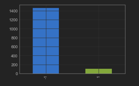
This data which is collected by these sensors not only contains relevant information but also a lot of noise. The dataset contains readings from 590. Among the 1567 examples, there are only 104 fail cases which means that out target variable is imbalanced. We will look at the distribution of the dataset when we look at the python code.

NOTE: For a detailed description regarding this cases study I highly recommend to read the following research papers:

  •  Kerdprasop, K., & Kerdprasop, N. A Data Mining Approach to Automate Fault Detection Model Development in the Semiconductor Manufacturing Process.
  • Munirathinam, S., & Ramadoss, B. Predictive Models for Equipment Fault Detection in the Semiconductor Manufacturing Process.

Data Understanding and Preparation

Let’s start exploring the dataset now. The first step as always is to import the required libraries.

import pandas as pd
import numpy as np

There are several ways to import the dataset, you can always download and then import from your working directory. However, I will directly import using the link. There are two datasets: one contains the readings from the sensors and the other one contains our target variable and a timestamp.

# Load dataset
url = "https://archive.ics.uci.edu/ml/machine-learning-databases/secom/secom.data"
names = ["feature" + str(x) for x in range(1, 591)]
secom_var = pd.read_csv(url, sep=" ", names=names, na_values = "NaN") 


url_l = "https://archive.ics.uci.edu/ml/machine-learning-databases/secom/secom_labels.data"
secom_labels = pd.read_csv(url_l,sep=" ",names = ["classification","date"],parse_dates = ["date"],na_values = "NaN")

The first step before doing the analysis would be to merge the dataset and we will us pandas library to merge the datasets in just one line of code.

#Data cleaning
#1. Combined the two datasets
secom_merged = pd.merge(secom_var, secom_labels,left_index=True,right_index=True)

Now let’s check out the distribution of the target variable

secom_merged.target.value_counts().plot(kind = 'bar')

Figure 1: Distribution of Target Variable

From Figure 1 it can be observed that the target variable is imbalanced and it is highly recommended to deal with this problem before the model building phase to avoid bias model. Xgboost is one of the models which can deal with imbalance classes but one needs to spend a lot of time to tune the hyper-parameters to achieve the best from the model.

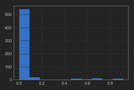
The dataset in hand contains a lot of null values and the next step would be to analyse these null values and remove the columns having null values more than a certain percentage. This percentage is calculated based on 95th quantile of null values.

#2. Analyzing nulls
secom_rmNa.isnull().sum().sum()
secom_nulls = secom_rmNa.isnull().sum()/len(secom_rmNa)
secom_nulls.describe()
secom_nulls.hist()

Figure 2: Missing percentge in each column

Now we calculate the 95th percentile of the null values.

x = secom_nulls.quantile(0.95)
secom_rmNa = secom_merged[secom_merged.columns[secom_nulls < x]]

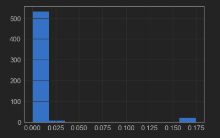
Figure 3: Missing percentage after removing columns with more then 45% Na

From figure 3 its visible that there are still missing values in the dataset and can be dealt by using many imputation methods. The most common method is to impute these values by mean, median or mode. There also exist few sophisticated techniques like K-nearest neighbour and interpolation.  We will be applying interpolation technique to our dataset. 

secom_complete = secom_rmNa.interpolate()

To prepare our dataset for analysis we should remove some more unwanted columns like columns with near zero variance. For this we can calulate number of unique values in each column and if there is only one unique value we can delete the column as it holds no information.

df = secom_complete.loc[:,secom_complete.apply(pd.Series.nunique) != 1]

## Let's check the shape of the df
df.shape
(1567, 444)

We have applied few data cleaning techniques and reduced the features from 590 to 444. However, In the next article we will apply some feature engineering techniques and adress problems like the curse of dimensionality and will also try to balance the target variable.

Bleiben Sie dran!!