Posts

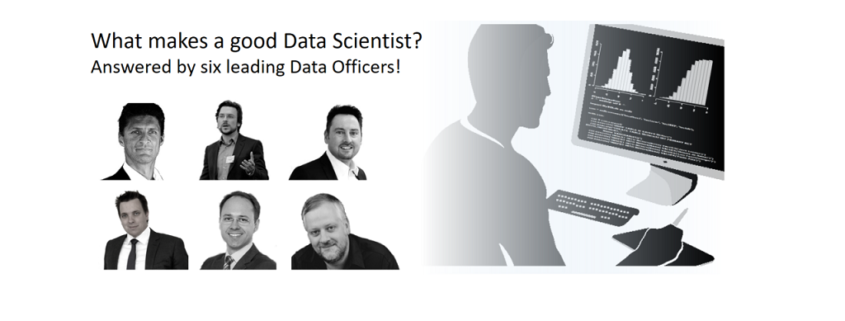
What makes a good Data Scientist? Answered by leading Data Officers!

What makes a good Data Scientist? A question I got asked recently a lot by data science newbies as well as long-established CIOs and my answer ist probably not what you think:
In my opinion is a good Data Scientist somebody with, at least, a good knowledge of computer programming, statistics and the ability of understanding the customer´s business. Above all stands a strong interest in finding value in distributed data sources.

Debatable? Maybe. That’s why I forwarded this question to five other leading Data Scientists and Chief Data Officers in Germany, let’s have a look on their answers to this question and create your own idea of what a good Data Scientist might be:


Dr. Andreas Braun – Head of Global Data & Analytics @ Allianz SE

A data scientist connects thorough analytical and methodological understanding  with a technical hands-on/ engineering mentality.
Data scientists bridge between analytics, tech, and business. “New methods”, such as machine learning, AI, deep learning etc. are crucial and are continuously challenged and improved. (14 February 2017)


Dr. Helmut Linde – Head of Data Science @ SAP SE

The ideal data scientist is a thought leader who creates value from analytics, starting from a vision for improved business processes and an algorithmic concept, down to the technical realization in productive software. (09 February 2017)


Klaas Bollhoefer – Chief Data Scientist @ The unbelievable Machine Company

For me a data scientist thinks ahead, thinks about and thinks in-between. He/she is a motivated, open-minded, enthusiastic and unconventional problem solver and tinkerer. Being a team player and a lone wolf are two sides of the same coin and he/she definitely hates unicorns and nerd shirts. (27 March 2017)


Wolfgang Hauner – Chief Data Officer @ Munich Re

A data scientist is, from their very nature, interested in data and its underlying relationship and has the cognitive, methodical and technical skills to find these relationships, even in unstructured data. The essential prerequisites to achieve this are curiosity, a logical mind-set and a passion for learning, as well as an affinity for team interaction in the work place. (08 February 2017)


Dr. Florian Neukart – Principal Data Scientist @ Volkswagen Group of America

In my opinion, the most important trait seems to be driven by an irresistible urge to understand fundamental relations and things, whereby I summarize both an atom and a complex machine among “things”. People with this trait are usually persistent, can solve a new problem even with little practical experience, and strive for the necessary training or appropriate quantitative knowledge autodidactically. (08 February 2017)

Background idea:
That I am writing about atoms and complex machines has to do with the fact that I have been able to analyze the most varied data through my second job at the university, and that I am given a chance to making significant contributions to both machine learning and physics, is primarily rooted in curiosity. Mathematics, physics, neuroscience, computer science, etc. are the fundamentals that someone will acquire if she wants to understand. In the beginning, there is only curiosity… I hope this is not too out of the way, but I’ve done a lot of job interviews and worked with lots of smart people, and it has turned out that quantitative knowledge alone is not enough. If someone is not burning for understanding, she may be able to program a Convolutional Network from the ground but will not come up with new ideas.


Statistical Relational Learning – Part 2

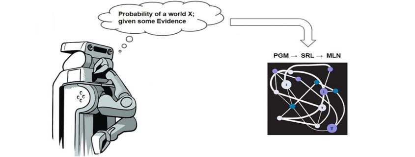
In the first part of this series onAn Introduction to Statistical Relational Learning”, I touched upon the basic Machine Learning paradigms, some background and intuition of the concepts and concluded with how the MLN template looks like. In this blog, we will dive in to get an in depth knowledge on the MLN template; again with the help of sample examples. I would then conclude by highlighting the various toolkit available and some of its differentiating features.

MLN Template – explained

A Markov logic network can be thought of as a group of formulas incorporating first-order logic and also tied with a weight. But what exactly does this weight signify?

Weight Learning

According to the definition, it is the log odds between a world where F is true and a world where F is false,

and captures the marginal distribution of the corresponding predicate.

Each formula can be associated with some weight value, that is a positive or negative real number. The higher the value of weight, the stronger the constraint represented by the formula. In contrast to classical logic, all worlds (i.e., Herbrand Interpretations) are possible with a certain probability [1]. The main idea behind this is that the probability of a world increases as the number of formulas it violates decreases.

Markov logic networks with its probabilistic approach combined to logic posit that a world is less likely if it violates formulas unlike in pure logic where a world is false if it violates even a single formula. Consider the case when a formula with high weight i.e. more significance is violated implying that it is less likely in occurrence.

Another important concept during the first phase of Weight Learning while applying an MLN template is “Grounding”. Grounding means to replace each variable/function in predicate with constants from the domain.

Weight Learning – An Example

Note: All examples are highlighted in the Alchemy MLN format

Let us consider an example where we want to identify the relationship between 2 different types of verb-noun pairs i.e noun subject and direct object.

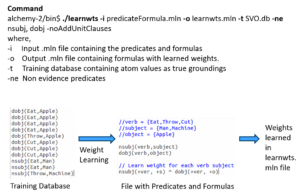
The input predicateFormula.mln file contains

  1. The predicates nsubj(verb, subject) and dobj(verb, object) and
  2. Formula of nsubj(+ver, +s) and dobj(+ver, +o)

These predicates or rules are to learn all possible SVO combinations i.e. what is the probability of a Subject-Verb-Object combination. The + sign ensures a cross product between the domains and learns all combinations. The training database consists of the nsubj and dobj tuples i.e. relations is the evidence used to learn the weights.

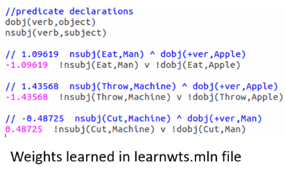
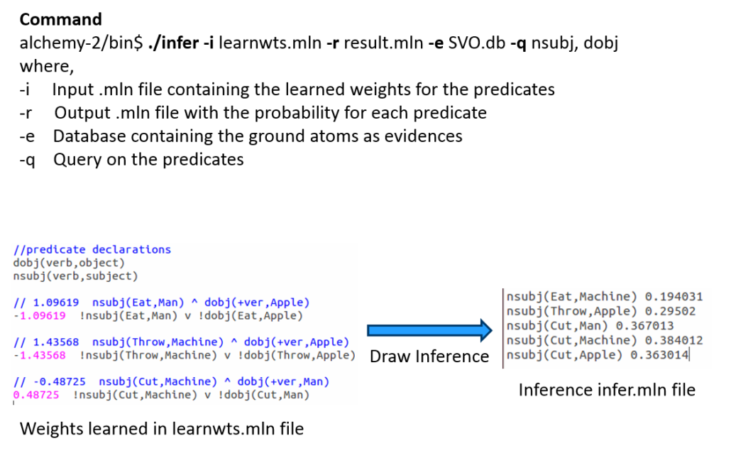
When we run the above command for this set of rules against the training evidence, we learn the weights as here:

Note that the formula is now grounded by all occurrences of nsubj and dobj tuples from the training database or evidence and the weights are attached to it at the start of each such combination.

But it should be noted that there is no network yet and this is just a set of weighted first-order logic formulas. The MLN template we created so far will generate Markov networks from all of our ground formulas. Internally, it is represented as a factor graph.where each ground formula is a factor and all the ground predicates found in the ground formula are linked to the factor.

Inference

The definition goes as follows:

Estimate probability distribution encoded by a graphical model, for a given data (or observation).

Out of the many Inference algorithms, the two major ones are MAP & Marginal Inference. For example, in a MAP Inference we find the most likely state of world given evidence, where y is the query and x is the evidence.

which is in turn equivalent to this formula.

Another is the Marginal Inference which computes the conditional probability of query predicates, given some evidence. Some advanced inference algorithms are Loopy Belief Propagation, Walk-SAT, MC-SAT, etc.

The probability of a world is given by the weighted sum of all true groundings of a formula i under an exponential function, divided by the partition function Z i.e. equivalent to the sum of the values of all possible assignments. The partition function acts a normalization constant to get the probability values between 0 and 1.

Inference – An Example

Let us draw inference on the the same example as earlier.

After learning the weights we run inference (with or without partial evidence) and query the relations of interest (nsubj here), to get inferred values.

Tool-kits

Let’s look at some of the MLN tool-kits at disposal to do learning and large scale inference. I have tried to make an assorted list of all tools here and tried to highlight some of its main features & problems.

For example, BUGS i.e. Bayesian Logic uses a Swift Compiler but is Not relational! ProbLog has a Python wrapper and is based on Horn clauses but has No Learning feature. These tools were invented in the initial days, much before the present day MLN looks like.

ProbCog developed at Technical University of Munich (TUM) & the AI Lab at Bremen covers not just MLN but also Bayesian Logic Networks (BLNs), Bayesian Networks & ProLog. In fact, it is now GUI based. Thebeast gives a shell to analyze & inspect model feature weights & missing features.

Alchemy from University of Washington (UoW) was the 1st First Order (FO) probabilistic logic toolkit. RockIt from University of Mannheim has an online & rest based interface and uses only Conjunctive Normal Forms (CNF) i.e. And-Or format in its formulas.

Tuffy scales this up by using a Relational Database Management System (RDBMS) whereas Felix allows Large Scale inference! Elementary makes use of secondary storage and Deep Dive is the current state of the art. All of these tools are part of the HAZY project group at Stanford University.

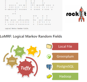
Lastly, LoMRF i.e. Logical Markov Random Field (MRF) is Scala based and has a feature to analyse different hypothesis by comparing the difference in .mln files!


Hope you enjoyed the read. The content starts from basic concepts and ends up highlighting key tools. In the final part of this 3 part blog series I would explain an application scenario and highlight the active research and industry players. Any feedback as a comment below or through a message is more than welcome!

Back to Part I – Statistical Relational Learning

Additional Links:

[1] Knowledge base files in Logical Markov Random Fields (LoMRF)

[2] (still) nothing clever Posts categorized “Machine Learning” – Markov Logic Networks

[3] A gentle introduction to statistical relational learning: maths, code, and examples

Success Criteria Process Mining

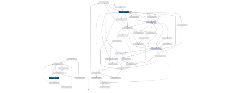
Process Mining is much more than the automatic drawing of process models.

Process mining is on the rise. By using Process mining, organizations can see how their processes really operate [1]. The results are amazing new insights about these processes that cannot be obtained in any other way. However, there are a few things that can go wrong. In this article, Frank van Geffen and Anne Rozinat give you tips about the pitfalls and advice that will help you to make your first process mining project as successful as it can be. Read more

Interview – Using Decision Science to forecast customer behaviour

Interview with Dr. Eva-Marie Müller-Stüler from KPMG about how to use Decision Science to forecast customer behaviour

Dr. Eva-Marie Müller-Stüler is Chief Data Scientist and Associate Director in Decision Science at KPMG LLP in London. She graduated as a mathematician at the Technical University of Munich with a year abroad in Tokyo, and completed her Doctorate at the Philipp University in Marburg.

linkedin-button xing-button

Read this article in German:
“Interview – Mit Data Science Kundenverhalten vorhersagen “

Data Science Blog: Ms Dr. Müller-Stüler, which path led you to the top of Analytics for KPMG?

I always enjoyed analytical questions, and have a great interest in people and finance. For me, understanding how people work and make decisions is incredibly exciting. In my Master’s and my PhD theses I had to analyse large amounts of data and had to program various algorithms. Now, combining a solid mathematical education with specific industry and business knowledge enables me to understand my clients’ businesses and to develop methods that disrupt the market and uncover new business strategies.

Data Science Blog: What kind of analytical solutions do you offer your clients? What benefits do you generate for them?

Our team focuses on Behaviour and Customer Science under a mantra and mission: “We understand human behaviour and we change it”. We look at all the data artefacts a person (for example, the customer or the employee) leaves behind and try to solve the question of how to change their behaviour or to predict future behaviour. With advanced analytics and data science we develop “always-on” forecasting models, which enable our clients to act in advance. This could be forecasting customer demand at a particular location, how it can be improved or influenced in the desired direction, or which kind of promotions work best for which customer. Also the challenge of predicting where, and with what product mix, a new store should be opened can be solved much more accurately with Predictive Analytics than by conventional methods.


Data Science Blog: What prerequisites must be fulfilled to ensure that predictive analyses work adequately for customer behaviour?

The data must, of course, have a certain quality and history to recognize trends and cycles. Often, however, one can also create an advantage by using additional new data sources. Experience and creativity are enormously important to understand what is possible and how to improve the quality of our work, or whether something only increases the noise.

Data Science Blog: What external data sources do you need to integrate? How do you handle unstructured data?

As far as external data sources are concerned, we are very spoiled here in England. We use about 10,000 different signals on average, and which vary depending on the question. These might include signals that show the composition of the population, local traffic information, the proximity of sights, hospitals, schools, crime rates and many more. The influence of each signal is also different for each problem. So, a high number of pick pocketing incidences can be a positive sign of the vibrancy of an area, and that people carry a lot of cash on average. For a fast food retailer with a presence in the city centre, for example, this could have a positive influence on a decision to invest in a new outlet in the area, in another area the opposite.

Data Science Blog: What possibilities does data science provide for forensics or fraud detection?

Every customer is surrounded by thousands of data signals and produces and transmits more by through his behaviour. This enables us to get a pretty good picture about the person online. As every kind of person also has a certain behavioural pattern (and this also applies to fraudsters) it is possible to recognise or predict these patterns in time.

Data Science Blog: What tools do you use in your work? When do you rely on proprietary software or on open source?

This depends on what stage we are in the process and the goal defined. We differentiate our team into different groups: Our Data Wranglers (who are responsible for extracting, generating and processing the data) work with other tools than our Data Modellers. Basically our tool kit covers the entire range of SQL Server, R, Python, but sometimes also Matlab or SAS. More and more, we are working with cloud-based solutions. Data visualization and dashboards in Qlik, Tableau or Alteryx are usually passed on to other teams.

Data Science Blog: What does your working day as a data scientist look like from after the morning café until the end of the evening?

My role is perhaps best described as the player’s coach. At the beginning of a project, it is primarily about working with the client to understand and develop the project. New ideas and methods have to be developed. During a project, I manage the teams and knowledge transfer; the review and the questioning of the models are my main tasks. In the end I do the final sign-off of the project. Since I often run several projects at different stages at the same time, it is guaranteed never boring.

Data Science Blog: Are good Data Scientists of your experience more likely to be consultant types or introvert nerds?

That depends upon what one is focused. A Data Visualizer or Data Artist reduces the information and visualise it in a great and understandable way. This requires creativity, a good understanding of business and safe handling of the tools.

The Data Analyst is more concerned with the “Slicing and Dicing” of data. The aim is to analyse the past and to recognize relationships. It is important to have good mathematical and statistical abilities in addition to the financial knowledge.

The Data Scientist is the most mathematical type. His job is to recognize deeper connections in the data and to make predictions. This involves the development of complicated models or Machine Learning Algorithms. Without a good mathematical education and programming skills it is unfortunately not possible to understand the risk of potential errors in full depth. The danger of drawing wrong conclusions or interpreting correlations counterfactually is very great. A simple example of this is that, in summer, when the weather is beautiful, more people eat ice cream and go swimming. Therefore, there is a strong correlation between eating ice and the number of drowned people, although eating ice cream does not lead to drowning. The influencing variable is the temperature. To minimise the risk for wrong conclusions I think it is important have worked and studied mathematics, data science, machine learning and statistics in depth – this usually means a PhD in science related subject.

Beyond that, business and industry knowledge is also important for a Data Scientist. His solutions must be relevant to the client and solve their problems or improve their processes. The best AI machine does not give any bank a competitive advantage if it predicts the sale of ice cream based on the weather. This may be 100% correct, but has no relevance for the client.

It is quite similar to other areas (e.g., medicine) too. There are many different areas, but for serious problems it is best to ask a specialist so that you do not draw wrong conclusions.

Data Science Blog: For all students who have soon finished their bachelor’s degree in computer science, mathematics, or economics, what would they advise these young ladies how to become good Data Scientists?

Never stop learning! The market is currently developing incredibly fast and has so many great areas to focus on. You should dive into it with passion, enthusiasm and creativity and have fun with the recognition of patterns and relationships. If you also surround yourself with interesting and inspiring people from whom you can learn more, I predict that you’ll do well.

This interview is also available in German: https://data-science-blog.com/de/blog/2016/11/10/interview-mit-advanced-analytics-kundenverhalten-verstehen/

Data Science on a large scale – can it be done?

Analytics drives business

In today’s digital world, data has become the crucial success factor for businesses as they seek to maintain a competitive advantage, and there are numerous examples of how companies have found smart ways of monetizing data and deriving value accordingly.

On the one hand, many companies use data analytics to streamline production lines, optimize marketing channels, minimize logistics costs and improve customer retention rates.  These use cases are often described under the umbrella term of operational BI, where decisions are based on data to improve a company’s internal operations, whether that be a company in the manufacturing industry or an e-commerce platform.

On the other hand, over the last few years, a whole range of new service-oriented companies have popped up whose revenue models wholly depend on data analytics.  These Data-Driven Businesses have contributed largely to the ongoing development of new technologies that make it possible to process and analyze large amounts of data to find the right insights.  The better these technologies are leveraged, the better their value-add and the better for their business success.  Indeed, without data and data analytics, they don’t have a business.

Data Science – hype or has it always been around?Druck

In my opinion, there is too much buzz around the new era of data scientists.  Ten years ago, people simply called it data mining, describing similar skills and methods.  What has actually changed is the fact that businesses are now confronted with new types of data sources such as mobile devices and data-driven applications rather than statistical methodologies.  I described that idea in detail in my recent post Let’s replace the Vs of Big Data with a single D.

But, of course, you cannot deny that the importance of these data crunchers has increased significantly. The art of mining data mountains (or perhaps I should say “diving through data lakes”) to find appropriate insights and models and then find the right answers to urgent, business-critical questions has become very popular these days.

The challenge: Data Science with large volumes?

Michael Stonebraker, winner of the Turing Award 2014, has been quoted as saying: “The change will come when business analysts who work with SQL on large amounts of data give way to data EXASOL Pipelinescientists, which will involve more sophisticated analysis, predictive modeling, regressions and Bayesian classification. That stuff at scale doesn’t work well on anyone’s engine right now. If you want to do complex analytics on big data, you have a big problem right now.”

And if you look at the limitations of existing statistical environments out there using R, Python, Java, Julia and other languages, I think he is absolutely right.  Once the data scientists have to handle larger volumes, the tools are just not powerful and scalable enough.  This results in data sampling or aggregation to make statistical algorithms applicable at all.

A new architecture for “Big Data Science”

We at EXASOL have worked hard to develop a smart solution to respond to this challenge.  Imagine that it is possible to use raw data and intelligent statistical models on very large data sets, directly at the place where the data is stored.  Where the data is processed in-memory to achieve optimal performance, all distributed across a powerful MPP cluster of servers, in an environment where you can now “install” the programming language of your choice.

Sounds far-fetched?  If you are not convinced, then I highly recommend you have a look at our brand-new in-database analytic programming platform, which is deeply integrated in our parallel in-memory engine and extensible through using nearly any programming language and statistical library.

For further information on our approach to big data science, go ahead and download a copy of our technical whitepaper:  Big Data Science – The future of analytics.

Neural Nets: Time Series Prediction

Artificial neural networks are very strong universal approximators. Google recently defeated the worlds strongest Go (“chinese chess”) player with two neural nets, which captured the game board as a picture. Aside from these classification tasks, neural nets can be used to predict future values, behaviors or patterns solely based on learned history. In the machine learning literature, this is often referred to as time series prediction, because, you know, values over time need to be predicted. Hah! To illustrate the concept, we will train a neural net to learn the shape of a sinusoidal wave, so it can continue to draw the shape without any help. We will do this with Scala. Scala is a great lang, because it is strongly typed but feels easy like Python. Throughout this article, I will use the library NeuroFlow, which is a simple, lightweight library I wrote to build and train nets. Because Open Source is the way to go, feel free to check (and contribute to? :-)) the code on GitHub.

Introduction of the shape

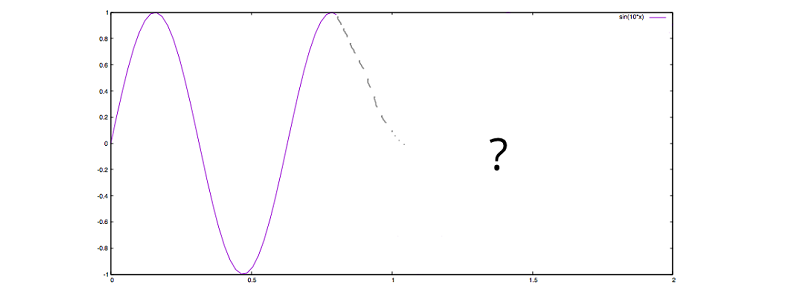
If we, as humans, want to predict the future based on historic observations, we would have no other chance but to be guided by the shape drawn so far. Let’s study the plot below, asking ourselves: How would a human continue the plot?

sinuspredictdr
f(x) = sin(10*x)

Intuitively, we would keep on oscillating up and down, just like the grey dotted line tries to rough out. To us, the continuation of the shape is reasonably easy to understand, but a machine does not have a gut feeling to ask for a good guess. However, we can summon a Frankenstein, which will be able to learn and continue the shape based on numbers. In order to do so, let’s have a look at the raw, discrete data of our sinusoidal wave:

x f(x)
0.0 0.0
0.05 0.479425538604203
0.10 0.8414709848078965
0.15 0.9974949866040544
0.20 0.9092974268256817
0.25 0.5984721441039564
0.30 0.1411200080598672
0.35 -0.35078322768961984
0.75 0.9379999767747389

Ranging from 0.0 until 0.75, these discrete values drawn from our function with step size 0.05 will be the basis for training. Now, one could come up with the idea to just memorize all values, so a sufficiently reasonable value can be picked based on comparison. For instance, to continue at the point 0.75 in our plot, we could simply examine the area close to 0.15, noticing a similar value close to 1, and hence go downwards. Well, of course this is cheating, but if a good cheat is a superior solution, why not cheat? Being hackers, we wouldn’t care. What’s really limiting here is the fact that the whole data set needs to be kept in memory, which can be infeasible for large sets, plus for more complex shapes, this approach would quickly result in a lot of weird rules and exceptions to be made in order to find comprehensible predictions.

Net to the rescue

Let’s go back to our table and see if a neural net can learn the shape, instead of simply memorizing it. Here, we want our net architecture to be of kind [3, 5, 3, 1]. Three input neurons, two hidden layers with five and three neurons respectively, as well as one neuron for the output layer will capture the data shown in the table.

sinuspredictnet

A supervised training mode means, that we want to train our net with three discrete steps as input and the fourth step as the supervised training element. So we will train a, b, c -> d and e, f, g -> h et cetera, hoping that this way our net will capture the slope pattern of our sinusoidal wave. Let’s code this in Scala:

import neuroflow.core.Activator.Tanh 
import neuroflow.core.WeightProvider.randomWeights 
import neuroflow.nets.DynamicNetwork.constructor

First, we want a Tanh activation function, because the domain of our sinusoidal wave is [-1, 1], just like the hyperbolic tangent. This way we can be sure that we are not comparing apples with oranges. Further, we want a dynamic network (adaptive learning rate) and random initial weights. Let’s put this down:

val fn = Tanh.apply
val sets = Settings(true, 10.0, 0.0000001, 500, None, None, Some(Map("τ" -> 0.25, "c" -> 0.25)))
val net = Network(Input(3) :: Hidden(5, fn) :: Hidden(3, fn) :: Output(1, fn) :: Nil, sets)

No surprises here. After some experiments, we can pick values for the settings instance, which will promise good convergence during training. Now, let’s prepare our discrete steps drawn from the sinus function:

val group = 4
val sinusoidal = Range.Double(0.0, 0.8, 0.05).grouped(group).toList.map(i => i.map(k => (k, Math.sin(10 * k))))
val xsys = sinusoidal.map(s => (s.dropRight(1).map(_._2), s.takeRight(1).map(_._2)))
val xs = xsys.map(_._1)
val ys = xsys.map(_._2)
net.train(xs, ys)

We will draw samples from the range with step size 0.05. After this, we will construct our training values xs as well as our supervised output values ys. Here, a group consists of 4 steps, with 3 steps as input and the last step as the supervised value.

[INFO] [25.01.2016 14:07:51:677] [run-main-5] Taking step 499 - error: 1.4395661497489177E-4  , error per sample: 3.598915374372294E-5
[INFO] [25.01.2016 14:07:51:681] [run-main-5] Took 500 iterations of 500 with error 1.4304189739640242E-4  
[success] Total time: 4 s, completed 25.01.2016 14:20:56

After a pretty short time, we will see good news. Now, how can we check if our net can successfully predict the sinusoidal wave? We can’t simply call our net like a sinus function to map from one input value to one output value, e. g. something like net(0.75) == sin(0.75). Our net does not care about any x values, because it was trained purely based on the function values f(x), or the slope pattern in general. We need to feed our net with a three-dimensional input vector holding the first three, original function values to predict the fourth step, then drop the first original step and append the recently predicted step to predict the fifth step, et cetera. In other words, we need to traverse the net. Let’s code this:

val initial = Range.Double(0.0, 0.15, 0.05).zipWithIndex.map(p => (p._1, xs.head(p._2)))
val result = predict(net, xs.head, 0.15, initial)
result.foreach(r => println(s"${r._1}, ${r._2}"))

with

@tailrec def predict(net: Network, last: Seq[Double], i: Double, results: Seq[(Double, Double)]): Seq[(Double, Double)] = {
  if (i < 4.0) {
    val score = net.evaluate(last).head
    predict(net, last.drop(1) :+ score, i + 0.05, results :+ (i, score))
  } else results
}

So, basically we don’t just continue to draw the sinusoidal shape at the point 0.75, we draw the entire shape right from the start until 4.0 – solely based on our trained net! Now, let’s see how our Frankenstein will complete the sinusoidal shape from 0.75 on:

sinuspredictfintwo

I’d say, pretty neat? Keep in mind, here, the discrete predictions are connected through splines. Another interesting property of our trained net is its prediction compared to the original sinus function when taking the limit towards 4.0. Let’s plot both:

sinuspredictfin

The purple line is the original sinusoidal wave, whereas the green line is the prediction of our net. The first steps show great consistency, but slowly the curves diverge a little over time, as uncertainties will add up. To keep this divergence rather low, one could fine tune settings, for instance numeric precision. However, if one is taking the limit towards infinity, a perfect fit is illusory.

Final thoughts

That’s it! We have trained our net to learn and continue the sinusoidal shape. Now, I know that this is a rather academic example, but to train a neural net to learn more complex shapes is straightforward from here.

Thanks for reading!

A quick primer on TensorFlow – Google’s machine learning workhorse

Introducing Google Brains‘ TensorFlow™

This week started with major news for the machine learning and data science community: the Google Brain Team announced the open sourcing of TensorFlow, their numerical library for tensor network computations. This software is actively developed (and used!) within Google and builds on many of Google’s large scale neural network applications such as automatic image labeling and captioning as well as the speech recognition in Google’s apps.

TensorFlow in bullet points

Here are the main features:

  • Supports deep neural networks – and much more machine learning approaches
  • Highly scalable across many machines and huge data sets
  • Runs on desktops, servers, in cloud and even mobile devices
  • Computation can run on CPUs, GPUs or both
  • All this flexibility is covered by a single API making the execution very streamlined
  • Available interfaces: C++ and Python. More will follow (Java, R, Lua, Go…)
  • Comes with many tools helping to build and visualize the data flow networks
  • Includes a powerful gradient based optimizer with auto-differentiation
  • Extensible with C++
  • Usable for commercial applications – released under Apache Software Licence 2.0

Tensor, what? Tensor, why?

„Numerical library for tensor network computations“ maybe doesn’t sound too exciting, but let’s  consider the implications.

Application of tensors and their networks is a relatively new (but fast evolving) approach in machine learning. Tensors, if you recall your algebra classes, are simply n-dimensional data arrays (so a scalar is a 0th order tensor, a vector is 1st order, and a matrix a 2nd order matrix).

A simple practical example of is color image’s RGB layers (essentially three 2D matrices combined into a 3rd order tensor). Or a more business minded example – if your data source generates a table (a 2D array) every hour, you can look at the full data set as a 3rd order tensor – time being the extra dimension.

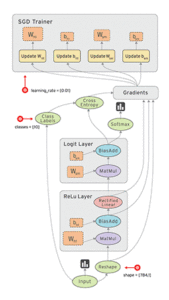
Tensor networks then represent “data flow graphs”, where the edges are your multi-dimensional data sets and nodes are the mathematical operations on this data.

Example of of a data flow graph with multiple nodes (data operations). Notice how the execution of nodes is asynchronous. This allows incredible scalability across many machines. Image Source.

Looking at your data through the tensor formalism gives you a lot of powerful tools that were already developed for tensor algebra, allowing fast, complex computations.  

Tensor networks are also a natural fit for computations done on graphical processing units (GPUs) as they are built exactly for the purpose of very fast numerical operations on such a data – speeding up your calculations significantly compared to standard CPU execution!

The importance of flexible architecture & scaling

The data flow graph approach has also further advantages. Most notably, you can split the design of your data flows (i.e. data cleaning, processing, transformations, model building etc.) from its execution. You first build up the graph of your data flow and then you send it to for execution: either on the CPUs of your machines (and it can be your laptop just as well as cluster) or GPUs or a combination. This happens through a single interface that hides all the complexities from you.

Since the execution is asynchronous it scales across many machines and can deal with huge amounts of data.

You can count on the Google guys to build tools not only for academic use, but also heavy-duty operations in the industry!

Is this just another deep learning library?

TensorFlow is of course not the first library to embrace the tensor formalism and GPU execution. The nearest comparisons (and competitors) are Theano, Torch and CGT (Caffe to a limited degree).

While there are significant overlaps between the libraries, TensorFlow tries to provide a broader framework. It is not only a deep learning library – the Data Flow Graphs can incorporate any data processing/analysis applications. It also comes with a very powerful gradient based optimizer with automatic calculations of derivatives offering huge flexibility.

Given this broad vision the closest competitor is probably Theano (while Caffe and the existing Theano wrappers have a narrower focus on deep learning). TensorFlow’s distinguishing feature is that by design its focus is on large, scalable architectures with a complete flexibility in the hardware, best suited for industry/operational use, whereas the other libraries have more academic pedigrees.

Initial analyses also indicate that TensorFlow should bring also performance improvements compared to Theano, although no comprehensive benchmarks have yet been published.

As the other packages are out already for a while, they have large, active communities and often additional supporting software (examples are the very useful wrappers around Theano like Lasagne, Keras and Blocks that provider higher level abstractions to its engine).

Of course, with Google’s gravitas, one can expect that TensorFlow’s open source community will grow very fast and the contributors will quickly add a lot of additional features (and find hidden bugs).

Finally, keep in mind, that while Google provided us with this great data processing framework and some of its machine learning capabilities, it is likely that the most powerful machine learning algorithms still remain Google’s proprietary secret.

Nonetheless, TensorFlow is a huge and very welcome contribution to the open source machine learning world!

Where to go next?

You can find Google’s getting started guide here. The TensorFlow white paper is worth a read too. Source code can be found at the Github page. There is also a Vagrant virtual machine with TensorFlow pre-installed available here.

Events

Nothing Found

Sorry, no posts matched your criteria