How To Remotely Send R and Python Execution to SQL Server from Jupyter Notebooks

Introduction

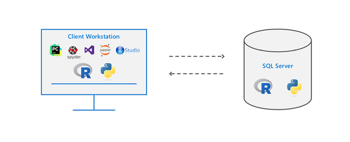
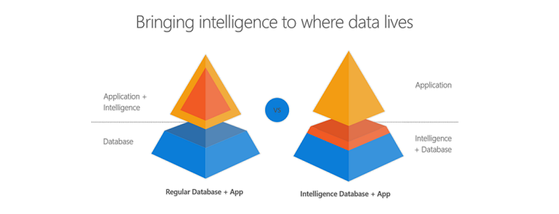
Did you know that you can execute R and Python code remotely in SQL Server from Jupyter Notebooks or any IDE? Machine Learning Services in SQL Server eliminates the need to move data around. Instead of transferring large and sensitive data over the network or losing accuracy on ML training with sample csv files, you can have your R/Python code execute within your database. You can work in Jupyter Notebooks, RStudio, PyCharm, VSCode, Visual Studio, wherever you want, and then send function execution to SQL Server bringing intelligence to where your data lives.
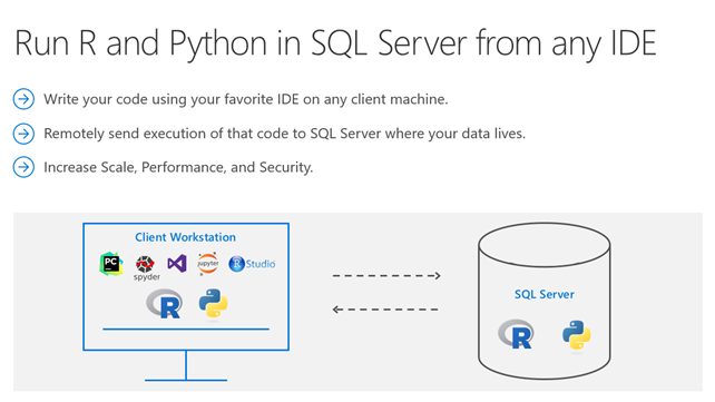
This tutorial will show you an example of how you can send your python code from Juptyter notebooks to execute within SQL Server. The same principles apply to R and any other IDE as well. If you prefer to learn through videos, this tutorial is also published on YouTube here:


Environment Setup Prerequisites

  1. Install ML Services on SQL Server

In order for R or Python to execute within SQL, you first need the Machine Learning Services feature installed and configured. See this how-to guide.

  1. Install RevoscalePy via Microsoft’s Python Client

In order to send Python execution to SQL from Jupyter Notebooks, you need to use Microsoft’s RevoscalePy package. To get RevoscalePy, download and install Microsoft’s ML Services Python Client. Documentation Page or Direct Download Link (for Windows).

After downloading, open powershell as an administrator and navigate to the download folder. Start the installation with this command (feel free to customize the install folder): .\Install-PyForMLS.ps1 -InstallFolder “C:\Program Files\MicrosoftPythonClient”

Be patient while the installation can take a little while. Once installed navigate to the new path you installed in. Let’s make an empty folder and open Jupyter Notebooks: mkdir JupyterNotebooks; cd JupyterNotebooks; ..\Scripts\jupyter-notebook

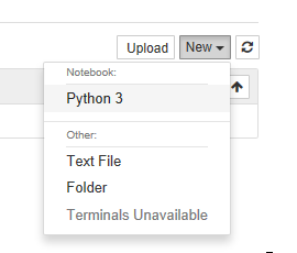
Create a new notebook with the Python 3 interpreter:
 

To test if everything is setup, import revoscalepy in the first cell and execute. If there are no error messages you are ready to move forward.

Database Setup (Required for this tutorial only)

For the rest of the tutorial you can clone this Jupyter Notebook from Github if you don’t want to copy paste all of the code. This database setup is a one time step to ensure you have the same data as this tutorial. You don’t need to perform any of these setup steps to use your own data.

  1. Create a database

Modify the connection string for your server and use pyodbc to create a new database.

import pyodbc  
# creating a new db to load Iris sample in 
new_db_name = "MLRemoteExec" connection_string = "Driver=SQL Server;Server=localhost\MSSQLSERVER2017;Database={0};Trusted_Connection=Yes;" 

cnxn = pyodbc.connect(connection_string.format("master"), autocommit=True) 

cnxn.cursor().execute("IF EXISTS(SELECT * FROM sys.databases WHERE [name] = '{0}') DROP DATABASE {0}".format(new_db_name)) 

cnxn.cursor().execute("CREATE DATABASE " + new_db_name)

cnxn.close()

print("Database created") 
  1. Import Iris sample from SkLearn

Iris is a popular dataset for beginner data science tutorials. It is included by default in sklearn package.

from sklearn import datasetsimport pandas as pd
# SkLearn has the Iris sample dataset built in to the packageiris = datasets.load_iris()
df = pd.DataFrame(iris.data, columns=iris.feature_names)
  1. Use RecoscalePy APIs to create a table and load the Iris data

(You can also do this with pyodbc, sqlalchemy or other packages)

from revoscalepy import RxSqlServerData, rx_data_step
# Example of using RX APIs to load data into SQL table. You can also do this with pyodbc
table_ref = RxSqlServerData(connection_string=connection_string.format(new_db_name), table="Iris")rx_data_step(input_data = df, output_file = table_ref, overwrite = True)print("New Table Created: Iris")
print("Sklearn Iris sample loaded into Iris table")

Define a Function to Send to SQL Server

Write any python code you want to execute in SQL. In this example we are creating a scatter matrix on the iris dataset and only returning the bytestream of the .png back to Jupyter Notebooks to render on our client.

def send_this_func_to_sql():
    from revoscalepy import RxSqlServerData, rx_import
    from pandas.tools.plotting import scatter_matrix
    import matplotlib.pyplot as plt
    import io    
# remember the scope of the variables in this func are within our SQL Server Python Runtime
    connection_string = "Driver=SQL Server;Server=localhost\MSSQLSERVER2017; Database=MLRemoteExec;Trusted_Connection=Yes;"

# specify a query and load into pandas dataframe df
    sql_query = RxSqlServerData(connection_string=connection_string, sql_query = "select * from Iris")

    df = rx_import(sql_query)
    scatter_matrix(df)

# return bytestream of image created by scatter_matrix
    buf = io.BytesIO()
    plt.savefig(buf, format="png")
    buf.seek(0)
    return buf.getvalue()

Send execution to SQL

Now that we are finally set up, check out how easy sending remote execution really is! First, import revoscalepy. Create a sql_compute_context, and then send the execution of any function seamlessly to SQL Server with RxExec. No raw data had to be transferred from SQL to the Jupyter Notebook. All computation happened within the database and only the image file was returned to be displayed.

from IPython import display
import matplotlib.pyplot as plt 
from revoscalepy import RxInSqlServer, rx_exec# create a remote compute context with connection to SQL Server

sql_compute_context = RxInSqlServer(connection_string=connection_string.format(new_db_name))

# use rx_exec to send the function execution to SQL Server

image = rx_exec(send_this_func_to_sql, compute_context=sql_compute_context)[0]

# only an image was returned to my jupyter client. All data remained secure and was manipulated in my db.

display.Image(data=image)

While this example is trivial with the Iris dataset, imagine the additional scale, performance, and security capabilities that you now unlocked. You can use any of the latest open source R/Python packages to build Deep Learning and AI applications on large amounts of data in SQL Server. We also offer leading edge, high-performance algorithms in Microsoft’s RevoScaleR and RevoScalePy APIs. Using these with the latest innovations in the open source world allows you to bring unparalleled selection, performance, and scale to your applications.

Learn More

Check out SQL Machine Learning Services Documentation to learn how you can easily deploy your R/Python code with SQL stored procedures making them accessible in your ETL processes or to any application. Train and store machine learning models in your database bringing intelligence to where your data lives.

Other YouTube Tutorials:

Bringing intelligence to where data lives: Python & R embedded in T-SQL

Introduction

Did you know that you can write R and Python code within your T-SQL statements? Machine Learning Services in SQL Server eliminates the need for data movement. Instead of transferring large and sensitive data over the network or losing accuracy with sample csv files, you can have your R/Python code execute within your database. Easily deploy your R/Python code with SQL stored procedures making them accessible in your ETL processes or to any application. Train and store machine learning models in your database bringing intelligence to where your data lives.

You can install and run any of the latest open source R/Python packages to build Deep Learning and AI applications on large amounts of data in SQL Server. We also offer leading edge, high-performance algorithms in Microsoft’s RevoScaleR and RevoScalePy APIs. Using these with the latest innovations in the open source world allows you to bring unparalleled selection, performance, and scale to your applications.

If you are excited to try out SQL Server Machine Learning Services, check out the hands on tutorial below. If you do not have Machine Learning Services installed in SQL Server,you will first want to follow the getting started tutorial I published here: 

How-To Tutorial

In this tutorial, I will cover the basics of how to Execute R and Python in T-SQL statements. If you prefer learning through videos, I also published the tutorial on YouTube.

Basics

Open up SQL Server Management Studio and make a connection to your server. Open a new query and paste this basic example: (While I use Python in these samples, you can do everything with R as well)

EXEC sp_execute_external_script @language = N'Python',
@script = N'print(3+4)'

Sp_execute_external_script is a special system stored procedure that enables R and Python execution in SQL Server. There is a “language” parameter that allows us to choose between Python and R. There is a “script” parameter where we can paste R or Python code. If you do not see an output print 7, go back and review the setup steps in this article.

Parameter Introduction

Now that we discussed a basic example, let’s start adding more pieces:

EXEC sp_execute_external_script  @language =N'Python', 
@script = N' 
OutputDataSet = InputDataSet;
',
@input_data_1 =N'SELECT 1 AS Col1';

Machine Learning Services provides more natural communications between SQL and R/Python with an input data parameter that accepts any SQL query. The input parameter name is called “input_data_1”.
You can see in the python code that there are default variables defined to pass data between Python and SQL. The default variable names are “OutputDataSet” and “InputDataSet” You can change these default names like this example:

EXEC sp_execute_external_script  @language =N'Python', 
@script = N' 
MyOutput = MyInput;
',
@input_data_1_name = N'MyInput',
@input_data_1 =N'SELECT 1 AS foo',
@output_data_1_name =N'MyOutput';

As you executed these examples, you might have noticed that they each return a result with “(No column name)”? You can specify a name for the columns that are returned by adding the WITH RESULT SETS clause to the end of the statement which is a comma separated list of columns and their datatypes.

EXEC sp_execute_external_script  @language =N'Python', 
@script=N' 
MyOutput = MyInput;
',
@input_data_1_name = N'MyInput',
@input_data_1 =N'
SELECT 1 AS foo,
2 AS bar
',
@output_data_1_name =N'MyOutput'
WITH RESULT SETS ((MyColName int, MyColName2 int));

Input/Output Data Types

Alright, let’s discuss a little more about the input/output data types used between SQL and Python. Your input SQL SELECT statement passes a “Dataframe” to python relying on the Python Pandas package. Your output from Python back to SQL also needs to be in a Pandas Dataframe object. If you need to convert scalar values into a dataframe here is an example:

EXEC sp_execute_external_script  @language =N'Python', 
@script=N' 
import pandas as pd
c = 1/2
d = 1*2
s = pd.Series([c,d])
df = pd.DataFrame(s)
OutputDataSet = df
'

Variables c and d are both scalar values, which you can add to a pandas Series if you like, and then convert them to a pandas dataframe. This one shows a little bit more complicated example, go read up on the python pandas package documentation for more details and examples:

EXEC sp_execute_external_script  @language =N'Python', 
@script=N' 
import pandas as pd
s = {"col1": [1, 2], "col2": [3, 4]}
df = pd.DataFrame(s)
OutputDataSet = df
'

You now know the basics to execute Python in T-SQL!

Did you know you can also write your R and Python code in your favorite IDE like RStudio and Jupyter Notebooks and then remotely send the execution of that code to SQL Server? Check out these documentation links to learn more: https://aka.ms/R-RemoteSQLExecution https://aka.ms/PythonRemoteSQLExecution

Check out the SQL Server Machine Learning Services documentation page for more documentation, samples, and solutions. Check out these E2E tutorials on github as well.

Would love to hear from you! Leave a comment below to ask a question, or start a discussion!

Statistical Relational Learning – Part 2

In the first part of this series onAn Introduction to Statistical Relational Learning”, I touched upon the basic Machine Learning paradigms, some background and intuition of the concepts and concluded with how the MLN template looks like. In this blog, we will dive in to get an in depth knowledge on the MLN template; again with the help of sample examples. I would then conclude by highlighting the various toolkit available and some of its differentiating features.

MLN Template – explained

A Markov logic network can be thought of as a group of formulas incorporating first-order logic and also tied with a weight. But what exactly does this weight signify?

Weight Learning

According to the definition, it is the log odds between a world where F is true and a world where F is false,

and captures the marginal distribution of the corresponding predicate.

Each formula can be associated with some weight value, that is a positive or negative real number. The higher the value of weight, the stronger the constraint represented by the formula. In contrast to classical logic, all worlds (i.e., Herbrand Interpretations) are possible with a certain probability [1]. The main idea behind this is that the probability of a world increases as the number of formulas it violates decreases.

Markov logic networks with its probabilistic approach combined to logic posit that a world is less likely if it violates formulas unlike in pure logic where a world is false if it violates even a single formula. Consider the case when a formula with high weight i.e. more significance is violated implying that it is less likely in occurrence.

Another important concept during the first phase of Weight Learning while applying an MLN template is “Grounding”. Grounding means to replace each variable/function in predicate with constants from the domain.

Weight Learning – An Example

Note: All examples are highlighted in the Alchemy MLN format

Let us consider an example where we want to identify the relationship between 2 different types of verb-noun pairs i.e noun subject and direct object.

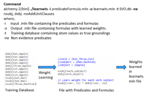
The input predicateFormula.mln file contains

  1. The predicates nsubj(verb, subject) and dobj(verb, object) and
  2. Formula of nsubj(+ver, +s) and dobj(+ver, +o)

These predicates or rules are to learn all possible SVO combinations i.e. what is the probability of a Subject-Verb-Object combination. The + sign ensures a cross product between the domains and learns all combinations. The training database consists of the nsubj and dobj tuples i.e. relations is the evidence used to learn the weights.

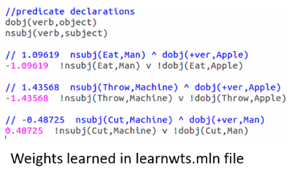
When we run the above command for this set of rules against the training evidence, we learn the weights as here:

Note that the formula is now grounded by all occurrences of nsubj and dobj tuples from the training database or evidence and the weights are attached to it at the start of each such combination.

But it should be noted that there is no network yet and this is just a set of weighted first-order logic formulas. The MLN template we created so far will generate Markov networks from all of our ground formulas. Internally, it is represented as a factor graph.where each ground formula is a factor and all the ground predicates found in the ground formula are linked to the factor.

Inference

The definition goes as follows:

Estimate probability distribution encoded by a graphical model, for a given data (or observation).

Out of the many Inference algorithms, the two major ones are MAP & Marginal Inference. For example, in a MAP Inference we find the most likely state of world given evidence, where y is the query and x is the evidence.

which is in turn equivalent to this formula.

Another is the Marginal Inference which computes the conditional probability of query predicates, given some evidence. Some advanced inference algorithms are Loopy Belief Propagation, Walk-SAT, MC-SAT, etc.

The probability of a world is given by the weighted sum of all true groundings of a formula i under an exponential function, divided by the partition function Z i.e. equivalent to the sum of the values of all possible assignments. The partition function acts a normalization constant to get the probability values between 0 and 1.

Inference – An Example

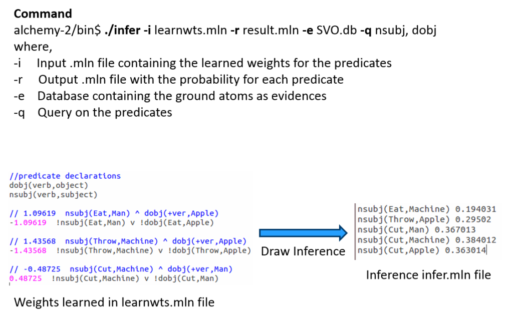
Let us draw inference on the the same example as earlier.

After learning the weights we run inference (with or without partial evidence) and query the relations of interest (nsubj here), to get inferred values.

Tool-kits

Let’s look at some of the MLN tool-kits at disposal to do learning and large scale inference. I have tried to make an assorted list of all tools here and tried to highlight some of its main features & problems.

For example, BUGS i.e. Bayesian Logic uses a Swift Compiler but is Not relational! ProbLog has a Python wrapper and is based on Horn clauses but has No Learning feature. These tools were invented in the initial days, much before the present day MLN looks like.

ProbCog developed at Technical University of Munich (TUM) & the AI Lab at Bremen covers not just MLN but also Bayesian Logic Networks (BLNs), Bayesian Networks & ProLog. In fact, it is now GUI based. Thebeast gives a shell to analyze & inspect model feature weights & missing features.

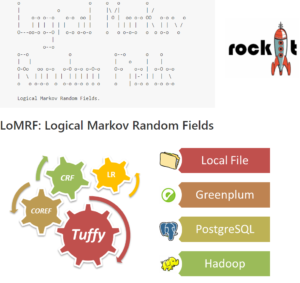
Alchemy from University of Washington (UoW) was the 1st First Order (FO) probabilistic logic toolkit. RockIt from University of Mannheim has an online & rest based interface and uses only Conjunctive Normal Forms (CNF) i.e. And-Or format in its formulas.

Tuffy scales this up by using a Relational Database Management System (RDBMS) whereas Felix allows Large Scale inference! Elementary makes use of secondary storage and Deep Dive is the current state of the art. All of these tools are part of the HAZY project group at Stanford University.

Lastly, LoMRF i.e. Logical Markov Random Field (MRF) is Scala based and has a feature to analyse different hypothesis by comparing the difference in .mln files!


Hope you enjoyed the read. The content starts from basic concepts and ends up highlighting key tools. In the final part of this 3 part blog series I would explain an application scenario and highlight the active research and industry players. Any feedback as a comment below or through a message is more than welcome!

Back to Part I – Statistical Relational Learning

Additional Links:

[1] Knowledge base files in Logical Markov Random Fields (LoMRF)

[2] (still) nothing clever Posts categorized “Machine Learning” – Markov Logic Networks

[3] A gentle introduction to statistical relational learning: maths, code, and examples

Neural Nets: Time Series Prediction

Artificial neural networks are very strong universal approximators. Google recently defeated the worlds strongest Go (“chinese chess”) player with two neural nets, which captured the game board as a picture. Aside from these classification tasks, neural nets can be used to predict future values, behaviors or patterns solely based on learned history. In the machine learning literature, this is often referred to as time series prediction, because, you know, values over time need to be predicted. Hah! To illustrate the concept, we will train a neural net to learn the shape of a sinusoidal wave, so it can continue to draw the shape without any help. We will do this with Scala. Scala is a great lang, because it is strongly typed but feels easy like Python. Throughout this article, I will use the library NeuroFlow, which is a simple, lightweight library I wrote to build and train nets. Because Open Source is the way to go, feel free to check (and contribute to? :-)) the code on GitHub.

Introduction of the shape

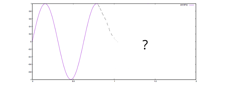
If we, as humans, want to predict the future based on historic observations, we would have no other chance but to be guided by the shape drawn so far. Let’s study the plot below, asking ourselves: How would a human continue the plot?

sinuspredictdr
f(x) = sin(10*x)

Intuitively, we would keep on oscillating up and down, just like the grey dotted line tries to rough out. To us, the continuation of the shape is reasonably easy to understand, but a machine does not have a gut feeling to ask for a good guess. However, we can summon a Frankenstein, which will be able to learn and continue the shape based on numbers. In order to do so, let’s have a look at the raw, discrete data of our sinusoidal wave:

x f(x)
0.0 0.0
0.05 0.479425538604203
0.10 0.8414709848078965
0.15 0.9974949866040544
0.20 0.9092974268256817
0.25 0.5984721441039564
0.30 0.1411200080598672
0.35 -0.35078322768961984
0.75 0.9379999767747389

Ranging from 0.0 until 0.75, these discrete values drawn from our function with step size 0.05 will be the basis for training. Now, one could come up with the idea to just memorize all values, so a sufficiently reasonable value can be picked based on comparison. For instance, to continue at the point 0.75 in our plot, we could simply examine the area close to 0.15, noticing a similar value close to 1, and hence go downwards. Well, of course this is cheating, but if a good cheat is a superior solution, why not cheat? Being hackers, we wouldn’t care. What’s really limiting here is the fact that the whole data set needs to be kept in memory, which can be infeasible for large sets, plus for more complex shapes, this approach would quickly result in a lot of weird rules and exceptions to be made in order to find comprehensible predictions.

Net to the rescue

Let’s go back to our table and see if a neural net can learn the shape, instead of simply memorizing it. Here, we want our net architecture to be of kind [3, 5, 3, 1]. Three input neurons, two hidden layers with five and three neurons respectively, as well as one neuron for the output layer will capture the data shown in the table.

sinuspredictnet

A supervised training mode means, that we want to train our net with three discrete steps as input and the fourth step as the supervised training element. So we will train a, b, c -> d and e, f, g -> h et cetera, hoping that this way our net will capture the slope pattern of our sinusoidal wave. Let’s code this in Scala:

import neuroflow.core.Activator.Tanh 
import neuroflow.core.WeightProvider.randomWeights 
import neuroflow.nets.DynamicNetwork.constructor

First, we want a Tanh activation function, because the domain of our sinusoidal wave is [-1, 1], just like the hyperbolic tangent. This way we can be sure that we are not comparing apples with oranges. Further, we want a dynamic network (adaptive learning rate) and random initial weights. Let’s put this down:

val fn = Tanh.apply
val sets = Settings(true, 10.0, 0.0000001, 500, None, None, Some(Map("τ" -> 0.25, "c" -> 0.25)))
val net = Network(Input(3) :: Hidden(5, fn) :: Hidden(3, fn) :: Output(1, fn) :: Nil, sets)

No surprises here. After some experiments, we can pick values for the settings instance, which will promise good convergence during training. Now, let’s prepare our discrete steps drawn from the sinus function:

val group = 4
val sinusoidal = Range.Double(0.0, 0.8, 0.05).grouped(group).toList.map(i => i.map(k => (k, Math.sin(10 * k))))
val xsys = sinusoidal.map(s => (s.dropRight(1).map(_._2), s.takeRight(1).map(_._2)))
val xs = xsys.map(_._1)
val ys = xsys.map(_._2)
net.train(xs, ys)

We will draw samples from the range with step size 0.05. After this, we will construct our training values xs as well as our supervised output values ys. Here, a group consists of 4 steps, with 3 steps as input and the last step as the supervised value.

[INFO] [25.01.2016 14:07:51:677] [run-main-5] Taking step 499 - error: 1.4395661497489177E-4  , error per sample: 3.598915374372294E-5
[INFO] [25.01.2016 14:07:51:681] [run-main-5] Took 500 iterations of 500 with error 1.4304189739640242E-4  
[success] Total time: 4 s, completed 25.01.2016 14:20:56

After a pretty short time, we will see good news. Now, how can we check if our net can successfully predict the sinusoidal wave? We can’t simply call our net like a sinus function to map from one input value to one output value, e. g. something like net(0.75) == sin(0.75). Our net does not care about any x values, because it was trained purely based on the function values f(x), or the slope pattern in general. We need to feed our net with a three-dimensional input vector holding the first three, original function values to predict the fourth step, then drop the first original step and append the recently predicted step to predict the fifth step, et cetera. In other words, we need to traverse the net. Let’s code this:

val initial = Range.Double(0.0, 0.15, 0.05).zipWithIndex.map(p => (p._1, xs.head(p._2)))
val result = predict(net, xs.head, 0.15, initial)
result.foreach(r => println(s"${r._1}, ${r._2}"))

with

@tailrec def predict(net: Network, last: Seq[Double], i: Double, results: Seq[(Double, Double)]): Seq[(Double, Double)] = {
  if (i < 4.0) {
    val score = net.evaluate(last).head
    predict(net, last.drop(1) :+ score, i + 0.05, results :+ (i, score))
  } else results
}

So, basically we don’t just continue to draw the sinusoidal shape at the point 0.75, we draw the entire shape right from the start until 4.0 – solely based on our trained net! Now, let’s see how our Frankenstein will complete the sinusoidal shape from 0.75 on:

sinuspredictfintwo

I’d say, pretty neat? Keep in mind, here, the discrete predictions are connected through splines. Another interesting property of our trained net is its prediction compared to the original sinus function when taking the limit towards 4.0. Let’s plot both:

sinuspredictfin

The purple line is the original sinusoidal wave, whereas the green line is the prediction of our net. The first steps show great consistency, but slowly the curves diverge a little over time, as uncertainties will add up. To keep this divergence rather low, one could fine tune settings, for instance numeric precision. However, if one is taking the limit towards infinity, a perfect fit is illusory.

Final thoughts

That’s it! We have trained our net to learn and continue the sinusoidal shape. Now, I know that this is a rather academic example, but to train a neural net to learn more complex shapes is straightforward from here.

Thanks for reading!