Posts

Geht mit Künstlicher Intelligenz nur „Malen nach Zahlen“?

Mit diesem Beitrag möchte ich darlegen, welche Grenzen uns in komplexen Umfeldern im Kontext Steuerung und Regelung auferlegt sind. Auf dieser Basis strebe ich dann nachgelagert eine Differenzierung in Bezug des Einsatzes von Data Science und Big Data, ab sofort mit Big Data Analytics bezeichnet, an. Aus meiner Sicht wird oft zu unreflektiert über Data Science und Künstliche Intelligenz diskutiert, was nicht zuletzt die Angst vor Maschinen schürt.

Basis meiner Ausführungen im ersten Part meines Beitrages ist der Kategorienfehler, der von uns Menschen immer wieder in Bezug auf Kompliziertheit und Komplexität vollführt wird. Deshalb werde ich am Anfang einige Worte über Kompliziertheit und Komplexität verlieren und dabei vor allem auf die markanten Unterschiede eingehen.

Kompliziertheit und Komplexität – der Versuch einer Versöhnung

Ich benutze oft die Begriffe „tot“ und „lebendig“ im Kontext von Kompliziertheit und Komplexität. Themenstellungen in „lebendigen“ Kontexten können niemals kompliziert sein. Sie sind immer komplex. Themenstellungen in „toten“ Kontexten sind stets kompliziert. Das möchte ich am Beispiel eines Uhrmachers erläutern, um zu verdeutlichen, dass auch Menschen in „toten“ Kontexten involviert sein können, obwohl sie selber lebendig sind. Deshalb die Begriffe „tot“ und „lebendig“ auch in Anführungszeichen.

Ein Uhrmacher baut eine Uhr zusammen. Dafür gibt es ein ganz klar vorgegebenes Rezept, welches vielleicht 300 Schritte beinhaltet, die in einer ganz bestimmten Reihenfolge abgearbeitet werden müssen. Werden diese Schritte befolgt, wird definitiv eine funktionierende Uhr heraus kommen. Ist der Uhrmacher geübt, hat er also genügend praktisches Wissen, ist diese Aufgabe für ihn einfach. Für mich als Ungelernten wird diese Übung schwierig sein, niemals komplex, denn ich kann ja einen Plan befolgen. Mit Übung bin ich vielleicht irgendwann so weit, dass ich diese Uhr zusammen gesetzt bekomme. Der Bauplan ist fix und ändert sich nicht. Man spricht hier von Monokontexturalität. Solche Tätigkeiten könnte man auch von Maschinen ausführen lassen, da klar definierte Abfolgen von Schritten programmierbar sind.

Nun stellen wir uns aber mal vor, dass eine Schraube fehlt. Ein Zahnrad kann nicht befestigt werden. Hier würde die Maschine einen Fehler melden, weil jetzt der Kontext verlassen wird. Das Fehlen der Schraube ist nicht Bestandteil des Kontextes, da es nicht Bestandteil des Planes und damit auch nicht Bestandteil des Programmcodes ist. Die Maschine weiß deshalb nicht, was zu tun ist. Der Uhrmacher ist in der Lage den Kontext zu wechseln. Er könnte nach anderen Möglichkeiten der Befestigung suchen oder theoretisch probieren, ob die Uhr auch ohne Zahnrad funktioniert oder er könnte ganz einfach eine Schraube bestellen und später den Vorgang fortsetzen. Der Uhrmacher kann polykontextural denken und handeln. In diesem Fall wird dann der komplizierte Kontext ein komplexer. Der Bauplan ist nicht mehr gültig, denn Bestellung einer Schraube war in diesem nicht enthalten. Deshalb meldet die Maschine einen Fehler. Der Bestellvorgang müsste von einem Menschen in Form von Programmcode voraus gedacht werden, so dass die Maschine diesen anstoßen könnte. Damit wäre diese Option dann wieder Bestandteil des monokontexturalen Bereiches, in dem die Maschine agieren kann.

Kommen wir in diesem Zusammenhang zum Messen und Wahrnehmen. Maschinen können messen. Messen passiert in monokontexturalen Umgebungen. Die Maschine kann messen, ob die Schraube festgezogen ist, die das Zahnrad hält: Die Schraube ist „fest“ oder „lose“. Im Falle des Fehlens der Schraube verlässt man die Ebene des Messens und geht in die Ebene der Wahrnehmung über. Die Maschine kann nicht wahrnehmen, der Uhrmacher schon. Beim Wahrnehmen muss man den Kontext erst einmal bestimmen, da dieser nicht per se gegeben sein kann. „Die Schraube fehlt“ setzt die Maschine in den Kontext „ENTWEDER fest ODER lose“ und dann ist Schluss. Die Maschine würde stetig zwischen „fest“ und „lose“ iterieren und niemals zum Ende gelangen. Eine endlose Schleife, die mit einem Fehler abgebrochen werden muss. Der Uhrmacher kann nach weiteren Möglichkeiten suchen, was gleichbedeutend mit dem Suchen nach einem weiteren Kontext ist. Er kann vielleicht eine neue Schraube suchen oder versuchen das Zahnrad irgendwie anders geartet zu befestigen.

In „toten“ Umgebungen ist der Mensch mit der Umwelt eins geworden. Er ist trivialisiert. Das ist nicht despektierlich gemeint. Diese Trivialisierung ist ausreichend, da ein Rezept in Form eines Algorithmus vorliegt, welcher zielführend ist. Wahrnehmen ist also nicht notwendig, da kein Kontextwechsel vorgenommen werden muss. Messen reicht aus.

In einer komplexen und damit „lebendigen“ Welt gilt das Motto „Sowohl-Als-Auch“, da hier stetig der Kontext gewechselt wird. Das bedeutet Widersprüchlichkeiten handhaben zu müssen. Komplizierte Umgebungen kennen ausschließlich ein „Entweder-Oder“. Damit existieren in komplizierten Umgebungen auch keine Widersprüche. Komplizierte Sachverhalte können vollständig in Programmcode oder Algorithmen geschrieben und damit vollständig formallogisch kontrolliert werden. Bei komplexen Umgebungen funktioniert das nicht, da unsere Zweiwertige Logik, auf die jeder Programmcode basieren muss, Widersprüche und damit Polykontexturalität ausschließen. Komplexität ist nicht kontrollier-, sondern bestenfalls handhabbar.

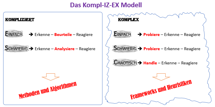
Diese Erkenntnisse möchte ich nun nutzen, um das bekannte Cynefin Modell von Dave Snowden zu erweitern, da dieses in der ursprünglichen Form zu Kategorienfehler zwischen Kompliziertheit und Komplexität verleitet. Nach dem Cynefin Modell werden die Kategorien „einfach“, „kompliziert“ und „komplex“ auf einer Ebene platziert. Das ist aus meiner Sicht nicht passfähig. Die Einstufung „einfach“ und damit auch „schwierig“, die es im Modell nicht gibt, existiert eine Ebene höher in beiden Kategorien, „kompliziert“ und „komplex“. „Einfach“ ist also nicht gleich „einfach“.

„Einfach“ in der Kategorie „kompliziert“ bedeutet, dass das ausreichende Wissen, sowohl praktisch als auch theoretisch, gegeben ist, um eine komplizierte Fragestellung zu lösen. Grundsätzlich ist ein Lösungsweg vorhanden, den man theoretisch kennen und praktisch anwenden muss. Wird eine komplizierte Fragestellung als „schwierig“ eingestuft, ist der vorliegende Lösungsweg nicht bekannt, aber grundsätzlich vorhanden. Er muss erlernt werden, sowohl praktisch als auch theoretisch. In der Kategorie „kompliziert“ rede ich also von Methoden oder Algorithmen, die an den bekannten Lösungsweg an-gelehnt sind.

Für „komplexe“ Fragestellungen kann per Definition kein Wissen existieren, welches in Form eines Rezeptes zu einem Lösungsweg geformt werden kann. Hier sind Erfahrung, Talent und Können essentiell, die Agilität im jeweiligen Kontext erhöhen. Je größer oder kleiner Erfahrung und Talent sind, spreche ich dann von den Wertungen „einfach“, „schwierig“ oder „chaotisch“. Da kein Rezept gegeben ist, kann man Lösungswege auch nicht vorweg in Form von Algorithmen programmieren. Hier sind Frameworks und Heuristiken angebracht, die genügend Freiraum für das eigene Denken und Fühlen lassen.

Die untere Abbildung stellt die Abhängigkeiten und damit die Erweiterung des Cynefin Modells dar.

Data Science und „lebendige“ Kontexte – der Versuch einer Versöhnung

Gerade beim Einsatz von Big Data Analytics sind wir dem im ersten Part angesprochenen Kategorienfehler erlegen, was mich letztlich zu einer differenzierten Sichtweise auf Big Data Analytics verleitet. Darauf komme ich nun zu sprechen.

In vielen Artikeln, Berichten und Büchern wird Big Data Analytics glorifiziert. Es gibt wenige Autoren, die eine differenzierte Betrachtung anstreben. Damit meine ich, klare Grenzen von Big Data Analytics, insbesondere in Bezug zum Einsatz auf Menschen, aufzuzeigen, um damit einen erfolgreichen Einsatz erst zu ermöglichen. Auch viele unserer Hirnforscher tragen einen erheblichen Anteil zum Manifestieren des Kategorienfehlers bei, da sie glauben, Wirkmechanismen zwischen der materiellen und der seelischen Welt erkundet zu haben. Unser Gehirn erzeugt aus dem Feuern von Neuronen, also aus Quantitäten, Qualitäten, wie „Ich liebe“ oder „Ich hasse“. Wie das funktioniert ist bislang unbekannt. Man kann nicht mit Algorithmen aus der komplizierten Welt Sachverhalte der komplexen Welt erklären. Die Algorithmen setzen auf der Zweiwertigen Logik auf und diese lässt keine Kontextwechsel zu. Ich habe diesen Fakt ja im ersten Teil eingehend an der Unterscheidung zwischen Kompliziertheit und Komplexität dargelegt.

Es gibt aber auch erfreulicherweise, leider noch zu wenige, Menschen, die diesen Fakt erkennen und thematisieren. Ich spreche hier stellvertretend Prof. Harald Walach an und zitiere aus seinem Artikel »Sowohl als auch« statt »Entweder-oder« – oder: wie man Kategorienfehler vermeidet.

„Die Wirklichkeit als Ganzes ist komplexer und lässt sich genau nicht mit solchen logischen Instrumenten komplett analysieren. … Weil unser Überleben als Art davon abhängig war, dass wir diesen logischen Operator so gut ausgeprägt haben ist die Gefahr groß dass wir nun alles so behandeln. … Mit Logik können wir nicht alle Probleme des Lebens lösen. … Geist und neuronale Entladungen sind Prozesse, die unterschiedlichen kategorialen Ebenen angehören, so ähnlich wie „blau“ und „laut“.

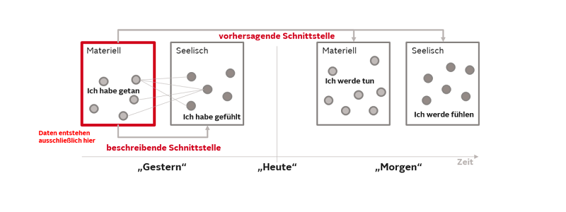
Aus diesen Überlegungen habe ich eine Big Data Analytics Matrix angefertigt, mit welcher man einen Einsatz von Big Data Analytics auf Menschen, also in „lebendige“ Kontexte, verorten kann.

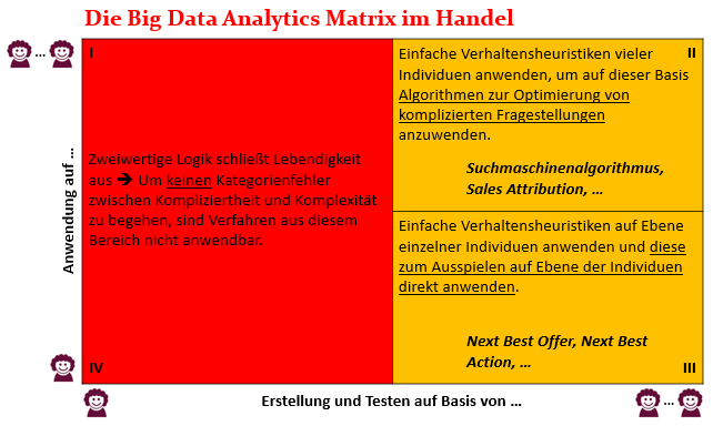
Die Matrix hat zwei Achsen. Die x-Achse stellt dar, auf welcher Basis, einzelne oder viele Menschen, Erkenntnisse direkt aus Daten und den darauf aufsetzenden Algorithmen gezogen werden sollen. Die y-Achse bildet ab, auf welcher Basis, einzelne oder viele Menschen, diese gewonnenen Erkenntnisse dann angewendet werden sollen. Um diese Unterteilung anschaulicher zu gestalten, habe ich in den jeweiligen Quadranten Beispiele eines möglichen Einsatzes von Big Data Analytics im Kontext Handel zugefügt.

An der Matrix erkennen wir, dass wir auf Basis von einzelnen Individuen keine Erkenntnisse maschinell über Algorithmen errechnen können. Tun wir das, begehen wir den von mir angesprochenen Kategorienfehler zwischen Kompliziertheit und Komplexität. In diesem Fall kennzeichne ich den gesamten linken roten Bereich der Matrix. Anwendungsfälle, die man gerne in diesen Bereich platzieren möchte, muss man über die anderen beiden gelben Quadranten der Matrix lösen.

Für das Lösen von Anwendungsfällen innerhalb der beiden gelben Quadranten kann man sich den Fakt zu Nutze machen, dass sich komplexe Vorgänge oft durch einfache Handlungsvorschriften beschreiben lassen. Achtung! Hier bitte nicht dem Versuch erlegen sein, „einfach“ und „einfach“ zu verwechseln. Ich habe im ersten Teil bereits ausgeführt, dass es sowohl in der Kategorie „kompliziert“, als auch in der Kategorie „komplex“, einfache Sachverhalte gibt, die aber nicht miteinander ob ihrer Schwierigkeitsstufe verglichen werden dürfen. Tut man es, dann, ja sie wissen schon: Kategorienfehler. Es ist ähnlich zu der Fragestellung: “Welche Farbe ist größer, blau oder rot?” Für Details hierzu verweise ich Sie gerne auf meinen Beitrag Komplexitäten entstehen aus Einfachheiten, sind aber schwer zu handhaben.

Möchten sie mehr zu der Big Data Analytics Matrix und den möglichen Einsätzen er-fahren, muss ich sie hier ebenfalls auf einen Beitrag von mir verweisen, da diese Ausführungen diesen Beitrag im Inhalt sprengen würden.

Mensch und Maschine – der Versuch einer Versöhnung

Wie Ihnen sicherlich bereits aufgefallen ist, enthält die Big Data Analytics Matrix keinen grünen Bereich. Den Grund dafür habe ich versucht, in diesem Beitrag aus meiner Sicht zu untermauern. Algorithmen, die stets monokontextural aufgebaut sein müssen, können nur mit größter Vorsicht im „lebendigen“ Kontext angewendet werden.

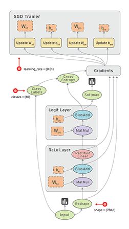
Erste Berührungspunkte in diesem Thema habe ich im Jahre 1999 mit dem Schreiben meiner Diplomarbeit erlangt. Die Firma, in welcher ich meine Arbeit verfasst habe, hat eine Maschine entwickelt, die aufgenommene Bilder aus Blitzgeräten im Straßenverkehr automatisch durchzieht, archiviert und daraus Mahnschreiben generiert. Ein Problem dabei war das Erkennen der Nummernschilder, vor allem wenn diese verschmutzt waren. Hier kam ich ins Spiel. Ich habe im Rahmen meiner Diplomarbeit ein Lernverfahren für ein Künstlich Neuronales Netz (KNN) programmiert, welches genau für diese Bilderkennung eingesetzt wurde. Dieses Lernverfahren setzte auf der Backpropagation auf und funktionierte auch sehr gut. Das Modell lag im grünen Bereich, da nichts in Bezug auf den Menschen optimiert werden sollte. Es ging einzig und allein um Bilderkennung, also einem „toten“ Kontext.

Diese Begebenheit war der Startpunkt für mich, kritisch die Strömungen rund um die Künstliche Intelligenz, vor allem im Kontext der Modellierung von Lebendigkeit, zu erforschen. Einige Erkenntnisse habe ich in diesem Beitrag formuliert.

Interview – Data Science in der Automobilbranche

Interview mit Herrn Dr. Florian Neukart, Principal Data Scientist der
Volkswagen Group of America

Herr Dr. Florian Neukart ist Principal Data Scientist der Volkswagen Group of America. Herr Neukart arbeitete nach seiner Promotion in der Informatik an der University of Brasov als Consultant für Business Analytics bei SAP und wechselte 2013 als Data Scientist zu Audi. 2015 übernahm er für mehr als ein Jahr die Funktion als Chief Technology Officer des Volkswagen Data Labs, bis er September 2016 zu Volkswagen in die USA wechselte. Darüber hinaus ist er bereits seit 2010 in der Forschung und Lehre für Quantum Computing, maschinelles Lernen und künstliche Intelligenz tätig und zudem Autor des Buches „Reverse Engineering the Mind – Consciously Acting Machines and Accelerated Evolution“.

Data Science Blog: Herr Dr. Neukart, Sie sind einer der führenden Data Scientists in der Automobilbranche. Schlägt Ihr Herz mehr für die automobile Praxis oder für die Forschung?

Das kann ich so klar nicht trennen – ich habe das Glück, seit Jahren in beiden Welten tätig sein zu können, und was für mich dabei den besonderen Reiz ausmacht, ist die Möglichkeit, neuste Forschung in die Praxis zu überführen, also anhand von realen Problemstellungen zu verifizieren, ob eine Theorie praxistauglich ist oder nicht. Umgekehrt gilt das genauso – es kommt vor, dass ich mich mit Fragestellungen konfrontiert sehe, für welche die erforderliche analytische Mathematik noch nicht entwickelt wurde, was wieder zu neuer Forschung und innovativen Ideen anregt. Schon mein ganzes Leben bin ich getrieben von Neugierde und will verstehen, wie Dinge funktionieren, unabängig davon, ob es sich um die Gruppendynamik und Selbstorganisation von Herzzellen, quantenphysikalisches Verhalten von subatomaren Teilchen, autonom agierende Fahrzeuge, Fluktuationsprognosen in Märkten oder die Auswertung und Interpretation von Sprache handelt. Dabei ist es zwar primär die Mathematik, die mir hilft, Zusammenhänge zu verstehen und zu interpretieren, aber erst die Technologien und Plattformen, die über die letzten Jahre entwickelt wurden, um etwa rechenintensive Mathematik zu parallelisieren, Daten im Hauptspeicher zu halten und effizient abzufragen, machen unsere Arbeit erst möglich und richtig interessant.

Data Science Blog: Welche Rolle spielt Data Science derzeit für die Automobilbranche? Sicherlich dreht sich gerade alles um das autonome Fahrzeug?

Natürlich sind selbstfahrende Fahrzeuge und Mobilität ein grosses Thema bei OEMs. Aber Data Science ist viel umfassender. Data Science hat bereits Einzug in die technische Entwicklung, Einkauf, Marketing, Logistik, Produktion, Sales, After Sales und Retail gehalten. Speziell der Connected Customer wird immer bedeutender, da sich die internationale Wettbewerbsfähigkeit in naher Zukunft auch über die neuen technischen und Serviceangebote definieren wird, die mit Hilfe von Data Science und maschinellem Lernen möglich werden. Bezogen auf selbstfahrende Fahrzeuge beginnen wir, das gesamte Ökosystem, bestehend aus Infrastruktur und unterschiedlichen Verkehrsteilnehmern, als Multi-Agentensystem zu betrachten. Vehicle to Vehicle und Vehicle to X-Kommunikation gewinnen an Bedeutung, und speziell die Einführung von sozialen Komponenten wird entscheidende Vorteile bringen. Beispielhaft gesprochen, können Ziele der Flotte sein, die Sicherheit für die Passagiere und andere Verkehrsteilnehmer (Passanten, Radfahrer, Motorräder, Fiaker :-)) zu maximieren und gleichzeitig den Verkehrsfluss zu optimieren. Es macht wenig Sinn, eine Ampel an einer Kreuzung auf Rot zu schalten, wenn die Kreuzung gefahrlos durchquert werden kann. Davon abgesehen werden in naher Zukunft alle Fahrzeuge mit ähnlichen Sensoren ausgestattet sein, etwa Kameras, LiDAR, Radar, Ultraschall und Mikrofonen zur akustischen Umfeldwahrnehmung. Ein weiteres Szenario versetzt die Stadtverwaltung in die Lage zu erkennen,  wo der Verkehrsfluss stockt und was getan werden muss, um diesen zu optimieren. Das „was getan werden muss“ ist extrem interessant – etwa könnte man die Strassen digital werden lassen, also Asphaltstraßen durch Glas ersetzen und durch OLEDs ergänzen. Damit sind dann dynamische Veränderungen der Verkehrsführung möglich. Materialtechnisch ist das machbar, denn die Oberflächenstruktur von Glas kann so entwickelt werden, dass dieses auch im Regen rutschfest ist. Glas kann zudem so flexibel und gleichzeitig stabil designet werden, dass auch darüberfahrende LKWs es nicht zum Brechen bringen. Die Abwärme der Displays kann zur Beheizung genutzt werden – es gibt somit auch im Winter keine Eisfahrbahnen mehr. Die Stadt kann sich selbst als Agent in die Multi-Agentenumgebung einbringen und zur Erreichung der definierten Ziele beitragen.

Data Science Blog: Was sind gerade heiße Themen im Automotive-Sektor? Und demgegenüber gestellt, welche Themen spielen in der KI-Forschung gerade eine größere Rolle?

Data Science hat in jedem Bereich Einzug gehalten. Jedes Thema ist auf seine Art „heiss“, egal ob es sich „nur“ um eine Marktprognose, die vorhin erwähnten Multi-Agentensysteme, kollaborative Arbeitsumgebungen, in denen Menschen und Roboter in der Produktion zusammenarbeiten, oder etwa persönliche Assistenten handelt. Nehmen wir eine Marktprognose als Beispiel. Hier sind für den menschlichen Entscheider nicht nur die internen Verkaufszahlen und alle Indikatoren, die etwa die Weltbank liefert, interessant, sondern auch die Gesellschaftsentwicklung und die politischen Strukturen.

In der KI-Forschung ist das für mich interessanteste Thema die generelle KI, also die Schaffung einer künstlichen Intelligenz, die domänenunabhängig komplexe Probleme selbstständig lösen kann. Vieles, was uns einfach scheint, hat sich aber als sehr komplex für KI-Systeme herausgestellt. Der Weg zur generellen KI und künstlichem Bewusstsein führt für mich über das Verständnis von Dingen, wobei ich hier sowohl ein Atom als auch eine komplexe Lebensform als „Ding“ zusammenfasse. Ein Teil, der uns (und Software) hilft, Dinge in deren Kontext und Umgebung einzubetten und zu beschreiben, ist die Sprache – etwa ist ein Reifen Teil eines Fahrzeugs und eine Schraube Teil eines Reifens. Das und die Kombinationen mit anderen Säulen der KI, wie etwa Computer Vision, Logik und Entscheidungsfindung, Maschine Learning und Multi-Agentensystemen (Multi-Agenten-Lernen), bringt uns der generellen und bewussten KI Schritt für Schritt näher, wobei ich mir hier nicht anmaße, eine Definition für Bewusstsein zu geben.

Data Science Blog: Welche Tools verwenden Sie bzw. Ihr Team bei Ihrer Arbeit? Setzen Sie dabei auch auf Open Source?

Wir sind „technolgieagnostisch“, wir versuchen also, für jeden Anwendungsfall die beste Technologie zu finden und einzusetzen. Das ist mal ein Tool oder eine Plattform von einem grossen Softwarehersteller, mal eine Lösung von einem Startup, wobei wir die meisten unserer Projekte doch in R oder Python umsetzen. Wir packen auch unsere Eigenentwicklungen in Libraries, die wir momentan aber noch ausschliesslich intern nutzen.


Data Science Blog: Was macht für Sie einen guten Data Scientist aus? Nach wem suchen Sie, wenn Sie einen Data Scientist einstellen?

Die wichtigste Eigenschaft scheint mir ein Drang nach dem Verständnis von Zusammenhängen und Dingen zu sein – eine starke Neugier – wobei ich unter „Dingen“ je nach Kontext Atome genauso wie komplexe Maschinen einordne.

Dass ich über Atome und komplexe Maschinen schreibe, hat damit zu tun, weil ich auch durch meinen zweiten Job an der Uni vielfältigste Daten analyiseren durfte. Und dass ich Beiträge zu Maschinenlernen und Physik verfasse, liegt tatsächlich in erster Linie an meiner Neugierde. Die Mathematik, Physik, Neurowissenschaft, Informatik … sind Grundlagen, die sich jemand aneignen wird, wenn sie/er verstehen will.

Data Science Blog: Wie sieht Ihrer Erfahrung nach der Arbeitsalltag als Data Scientist nach dem morgendlichen Café bis zum Feierabend aus?

Idealerweise startet der Tag nicht mit Emails :-). Wenn ich aus meiner Erfahrung sprechen darf, dann lässt einen die Data Science auch nach der Arbeit nicht los und die Grenzen von Beruf und Hobby überlagern sich irgendwann. Schon während dem morgendlichen Café tauschen wir uns über die jeweiligen Projekte aus – jeder sollte soviel wie möglich über alle Projekte wissen, um nicht lediglich Nischenwissen aufzubauen. Scrum hat sich auch in Bezug auf Data Science bewährt – je nachdem, wie viele Data Scientists an einem Thema arbeiten und wie viele Tasks anfallen, machen tägliche Stand-Ups Sinn – speziell wenn ein Projekt viele Subkomponenten hat, die als grosses Ganzes funktionieren müssen, hat so jeder Beteiligte immer vollste Transparenz. Die meiste Zeit fliesst natürlich in die Entwicklung der jeweiligen Prototypen / Produkte, aber etwa ein Drittel sollte reserviert sein für das Durcharbeiten von Papers mit aktuellsten Forschungsergebnissen und dem Einarbeiten in neue Technologien. Ich habe mal gesagt bekommen „Data Scientists sprechen nicht viel“, was für die Zeit während der Entwicklungsarbeit (und meiner Erfahrung nach auf die meisten Informatiker) auch zutrifft, da wir zumeist den Zustand eines komplexen Systems im Kopf behalten müssen – tatsächlich aber sprechen wir sehr gerne und viel über mögliche Arten, Probleme zu verstehen und zu lösen. Für meine Kollegen und mich ist Data Science kein bloßer Job, wir beschäftigen uns auch nach dem Feierabend noch mit relevanter Lektuere oder privaten Side-Projects – wie gesagt, wir haben das Glück, Job und Hobby zu vereinen.

Data Science Blog: Für alle Studenten, die demnächst ihren Bachelor, beispielsweise in Informatik, Mathematik oder Wirtschaftslehre, abgeschlossen haben, was würden sie diesen jungen Damen und Herren raten, wie sie einen guten Einstieg ins Data Science bewältigen können?

Natürlich ist ein solider methodischer Hintergrund, darunter Statistik, Mathematik und Informatik mit Fokus auf Machine Learning erforderlich, und auch das technische Wissen, die Theorie in Produkte zu überführen, also in Programmiersprachen und relevante Libraries, Datenbanken, Streaming und IoT. Das sind Kernkompetenzen, aber wie gesagt, am Anfang steht die Neugierde. Ich rate jedoch jedem, sich einem Problem nicht ausschließlich über die Theorie zu nähern, sondern erst zu versuchen, das Problem zu verstehen und das theoretische Wissen hands-on aufzubauen. Niemand weiss alles, und die Recherche rund um ein Problem ist ein wichtiger Lernprozess, aus dem man unglaublich viel mitnehmen kann. Data Science ist immer hands-on, und Neugierde führt zum Ziel.

Maschinelles Lernen mit Entscheidungsbaumverfahren – Artikelserie

Das Entscheidungsbaumverfahren (Decision Tree) ist eine verbreitete Möglichkeit der Regression oder Klassifikation über einen vielfältigen Datensatz. Das Verfahren wird beispielsweise dazu verwendet, um die Kreditwürdigkeit von Bankkunden zu klassifizieren oder auch, um eine Funktion zur Vorhersage einer Kaufkraft zu bilden.

Sicherlich hat beinahe jeder Software-Entwickler bereits einen Entscheidungsbaum (meistens binäre Baumstrukturen) programmiert und auch Maschinenbauingenieure benutzen Entscheidungsbäume, um Konstruktionsstrukturen darzustellen. Im Data Science haben Entscheidungsbäume allerdings eine etwas andere Bedeutung, denn ein Data Scientist befasst sich weniger mit dem manuellen Erstellen von solchen Baumstrukturen, sondern viel mehr mit Algorithmen, die ausreichend gute (manchmal: best mögliche) Baumstrukturen automatisch aus eine Menge mehr oder weniger bekannter Daten heraus generieren, die dann für eine automatische Klassifikation bzw. Regression dienen können.

Entscheidungsbäume sind also eine Idee des überwachten maschinellen Lernens, bei der Algorithmen zum Einsatz kommen, die aus einer Datenmenge heraus eine hierarchische Struktur von möglichst wenigen Entscheidungswegen bilden. Diese Datenmenge stellt eine sogenannte Trainingsstichprobe dar. Meiner Erfahrung nach werde Entscheidungsbäume oftmals in ihrer Mächtigkeit, aber auch in ihrer Komplexität unterschätzt und die Einarbeitung fiel mehr selbst schwerer, als ich anfangs annahm: In der Praxis stellt das Verfahren den Data Scientist vor viele Herausforderungen.

In dieser Artikelserie wird es vier nachfolgende Teile geben (Verlinkung erfolgt nach Veröffentlichung):


Statistical Relational Learning – Part 2

In the first part of this series onAn Introduction to Statistical Relational Learning”, I touched upon the basic Machine Learning paradigms, some background and intuition of the concepts and concluded with how the MLN template looks like. In this blog, we will dive in to get an in depth knowledge on the MLN template; again with the help of sample examples. I would then conclude by highlighting the various toolkit available and some of its differentiating features.

MLN Template – explained

A Markov logic network can be thought of as a group of formulas incorporating first-order logic and also tied with a weight. But what exactly does this weight signify?

Weight Learning

According to the definition, it is the log odds between a world where F is true and a world where F is false,

and captures the marginal distribution of the corresponding predicate.

Each formula can be associated with some weight value, that is a positive or negative real number. The higher the value of weight, the stronger the constraint represented by the formula. In contrast to classical logic, all worlds (i.e., Herbrand Interpretations) are possible with a certain probability [1]. The main idea behind this is that the probability of a world increases as the number of formulas it violates decreases.

Markov logic networks with its probabilistic approach combined to logic posit that a world is less likely if it violates formulas unlike in pure logic where a world is false if it violates even a single formula. Consider the case when a formula with high weight i.e. more significance is violated implying that it is less likely in occurrence.

Another important concept during the first phase of Weight Learning while applying an MLN template is “Grounding”. Grounding means to replace each variable/function in predicate with constants from the domain.

Weight Learning – An Example

Note: All examples are highlighted in the Alchemy MLN format

Let us consider an example where we want to identify the relationship between 2 different types of verb-noun pairs i.e noun subject and direct object.

The input predicateFormula.mln file contains

  1. The predicates nsubj(verb, subject) and dobj(verb, object) and
  2. Formula of nsubj(+ver, +s) and dobj(+ver, +o)

These predicates or rules are to learn all possible SVO combinations i.e. what is the probability of a Subject-Verb-Object combination. The + sign ensures a cross product between the domains and learns all combinations. The training database consists of the nsubj and dobj tuples i.e. relations is the evidence used to learn the weights.

When we run the above command for this set of rules against the training evidence, we learn the weights as here:

Note that the formula is now grounded by all occurrences of nsubj and dobj tuples from the training database or evidence and the weights are attached to it at the start of each such combination.

But it should be noted that there is no network yet and this is just a set of weighted first-order logic formulas. The MLN template we created so far will generate Markov networks from all of our ground formulas. Internally, it is represented as a factor graph.where each ground formula is a factor and all the ground predicates found in the ground formula are linked to the factor.

Inference

The definition goes as follows:

Estimate probability distribution encoded by a graphical model, for a given data (or observation).

Out of the many Inference algorithms, the two major ones are MAP & Marginal Inference. For example, in a MAP Inference we find the most likely state of world given evidence, where y is the query and x is the evidence.

which is in turn equivalent to this formula.

Another is the Marginal Inference which computes the conditional probability of query predicates, given some evidence. Some advanced inference algorithms are Loopy Belief Propagation, Walk-SAT, MC-SAT, etc.

The probability of a world is given by the weighted sum of all true groundings of a formula i under an exponential function, divided by the partition function Z i.e. equivalent to the sum of the values of all possible assignments. The partition function acts a normalization constant to get the probability values between 0 and 1.

Inference – An Example

Let us draw inference on the the same example as earlier.

After learning the weights we run inference (with or without partial evidence) and query the relations of interest (nsubj here), to get inferred values.

Tool-kits

Let’s look at some of the MLN tool-kits at disposal to do learning and large scale inference. I have tried to make an assorted list of all tools here and tried to highlight some of its main features & problems.

For example, BUGS i.e. Bayesian Logic uses a Swift Compiler but is Not relational! ProbLog has a Python wrapper and is based on Horn clauses but has No Learning feature. These tools were invented in the initial days, much before the present day MLN looks like.

ProbCog developed at Technical University of Munich (TUM) & the AI Lab at Bremen covers not just MLN but also Bayesian Logic Networks (BLNs), Bayesian Networks & ProLog. In fact, it is now GUI based. Thebeast gives a shell to analyze & inspect model feature weights & missing features.

Alchemy from University of Washington (UoW) was the 1st First Order (FO) probabilistic logic toolkit. RockIt from University of Mannheim has an online & rest based interface and uses only Conjunctive Normal Forms (CNF) i.e. And-Or format in its formulas.

Tuffy scales this up by using a Relational Database Management System (RDBMS) whereas Felix allows Large Scale inference! Elementary makes use of secondary storage and Deep Dive is the current state of the art. All of these tools are part of the HAZY project group at Stanford University.

Lastly, LoMRF i.e. Logical Markov Random Field (MRF) is Scala based and has a feature to analyse different hypothesis by comparing the difference in .mln files!


Hope you enjoyed the read. The content starts from basic concepts and ends up highlighting key tools. In the final part of this 3 part blog series I would explain an application scenario and highlight the active research and industry players. Any feedback as a comment below or through a message is more than welcome!

Back to Part I – Statistical Relational Learning

Additional Links:

[1] Knowledge base files in Logical Markov Random Fields (LoMRF)

[2] (still) nothing clever Posts categorized “Machine Learning” – Markov Logic Networks

[3] A gentle introduction to statistical relational learning: maths, code, and examples

Statistical Relational Learning

An Introduction to Statistical Relational Learning – Part 1

Statistical Relational Learning (SRL) is an emerging field and one that is taking centre stage in the Data Science age. Big Data has been one of the primary reasons for the continued prominence of this relational learning approach given, the voluminous amount of data available now to learn interesting and unknown patterns from data. Moreover, the tools have also improved their processing prowess especially, in terms of scalability.

This introductory blog is a prelude on SRL and later on I would also touch base on more advanced topics, specifically Markov Logic Networks (MLN). To start off, let’s look at how SRL fits into one of the 5 different Machine Learning paradigms.

Five Machine Learning Paradigms

Lets look at the 5 Machine Learning Paradigms: Each of which is inspired by ideas from a different field!

  1. Connectionists as they are called and led by Geoffrey Hinton (University of Toronto & Google and one of the major names in the Deep Learning community) think that a learning algorithm should mimic the brain! After all it is the brain that does all the complex actions for us and, this idea stems from Neuroscience.
  2. Another group of Evolutionists whose leader is the late John Holland (from the University of Michigan) believed it is not the brain but evolution that was precedent and hence the master algorithm to build anything. And using this approach of having the fittest ones program the future they are currently building 3D prints of future robots.
  3. Another thought stems from Philosophy where Analogists like Douglas R. Hofstadter an American writer and author of popular and award winning book – Gödel, Escher, Bach: an Eternal Golden Braid believe that Analogy is the core of Cognition.
  4. Symbolists like Stephen Muggleton (Imperial College London) think Psychology is the base and by developing Rules in deductive reasoning they built Adam – a robot scientist at the University of Manchester!
  5. Lastly we have a school of thought which has its foundations rested on Statistics & Logic, which is the focal point of interest in this blog. This emerging field has started to gain prominence with the invention of Bayesian networks 2011 by Judea Pearl (University of California Los Angeles – UCLA) who was awarded with the Turing award (the highest award in Computer Science). Bayesians as they are called, are the most fanatical of the lot as they think everything can be represented by the Bayes theorem using hypothesis which can be updated based on new evidence.

SRL fits into the last paradigm of Statistics and Logic. As such it offers another alternative to the now booming Deep Learning approach inspired from Neuroscience.

Background

In many real world scenario and use cases, often the underlying data is assumed to be independent and identically distributed (i.i.d.). However, real world data is not and instead consists of many relationships. SRL as such attempts to represent, model, and learn in the relational domain!

There are 4 main Models in SRL

  1. Probabilistic Relational Models (PRM)
  2. Markov Logic Networks (MLN)
  3. Relational Dependency Networks (RDN)
  4. Bayesian Logic Programs (BLP)

It is difficult to cover all major models and hence the focus of this blog is only on the emerging field of Markov Logic Networks.
MLN is a powerful framework that combines statistics (i.e. it uses Markov Random Fields) and logical reasoning (first order logic).


markov-random-fields-first-order-logic

Academia

Some of the prominent names in academic and the research community in MLN include:

  1. Professor Pedro Domingos from the University of Washington is credited with introducing MLN in his paper from 2006. His group created the tool called Alchemy which was one of the first, First Order Logic tools.
  2. Another famous name – Professor Luc De Raedt from the AI group at University of Leuven in Belgium, and their team created the tool ProbLog which also has a Python Wrapper.
  3. HAZY Project (Stanford University) led by Prof. Christopher Ré from the InfoLab is doing active research in this field and Tuffy, Felix, Elementary, Deep Dive are some of the tools developed by them. More on it later!
  4. Talking about academia close by i.e. in Germany, Prof. Michael Beetz and his entire team moved from TUM to TU Bremen. Their group invented the tool – ProbCog
  5. At present, Prof. Volker Tresp from Ludwig Maximilians University (LMU), Munich & Dr. Matthias Nickles at Technical University of Munich (TUM) have research interests in SRL.

Theory & Formulation

A look at some background and theoretical concepts to understand MLN better.

A. Basics – Probabilistic Graphical Models (PGM)

The definition of a PGM goes as such:

A PGM encodes a joint p(x,y) or conditional p(y|x) probability distribution such that given some observations we are provided with a full probability distribution over all feasible solutions.

A PGM helps to encode relationships between a set of random variables. And it achieves this by making use of a graph! These graphs can be either be Directed or Undirected Graphs.

B. Markov Blanket

A Markov Blanket is a Directed Acyclic graph. It is a Bayesian network and as you can see the central node A highlighted in red is dependent on its parents and parents of descendents (moralization) by the circle drawn around it. Thus these nodes are the only knowledge needed to predict node A.

C. Markov Random Fields (MRF)

A MRF is an Undirected graphical model. Every node in an MRF satisfies the Local Markov property of Conditional Independence, i.e. a node is conditionally independent of another node, given its neighbours. And now relating it to Markov Blanket as explained previously, a Markov blanket for a node is simply its adjacent nodes!

Intuition

We now that Probability handles uncertainty whereas Logic handles complexity. So why not make use of both of them to model relationships in data that is both uncertain and complex. Markov Logic Networks (MLN) precisely does that for us!

MLN is composed of a set of pairs of  <w, F> where F is the formula (written in FO logic) and weights (real numbers identifying the strength of the constraint).

MLN basically provides a template to ground a Markov network. Grounding would be explained in detail in the next but one section on “Weight Learning”.

It can be defined as a Log linear model where probability of a world is given by the weighted sum of all true groundings of a formula i under an exponential function. It is then divided by Z which is termed as the partition function and used to normalize and get probability values between 0 and 1.

propability_of_a_world_x

The MLN Template

Rules or Predicates

The relation to be learned is expressed in FO logic. Some of the different possible FO logical connectives and quantifiers are And (^), Or (V), Implication (→), and many more. Plus, Formulas may contain one or more predicates, connected to each other with logical connectives and quantified symbols.

Evidence

Evidence represent known facts i.e. the ground predicates. Each fact is expressed with predicates that contain only constants from their corresponding domains.

Weight Learning

Discover the importance of relations based on grounded evidence.

Inference

Query relations, given partial evidence to infer a probabilistic estimate of the world.

More on Weight Learning and Inference in the next part of this series!

Hope you enjoyed the read. I have deliberately kept the content basic and a mix of non technical and technical so as to highlight first the key players and some background concepts and generate the reader’s interest in this topic, the technicalities of which can easily be read in the paper. Any feedback as a comment below or through a message are more than welcome!

Continue reading with Statistical Relational Learning – Part II.

References

Neural Nets: Time Series Prediction

Artificial neural networks are very strong universal approximators. Google recently defeated the worlds strongest Go (“chinese chess”) player with two neural nets, which captured the game board as a picture. Aside from these classification tasks, neural nets can be used to predict future values, behaviors or patterns solely based on learned history. In the machine learning literature, this is often referred to as time series prediction, because, you know, values over time need to be predicted. Hah! To illustrate the concept, we will train a neural net to learn the shape of a sinusoidal wave, so it can continue to draw the shape without any help. We will do this with Scala. Scala is a great lang, because it is strongly typed but feels easy like Python. Throughout this article, I will use the library NeuroFlow, which is a simple, lightweight library I wrote to build and train nets. Because Open Source is the way to go, feel free to check (and contribute to? :-)) the code on GitHub.

Introduction of the shape

If we, as humans, want to predict the future based on historic observations, we would have no other chance but to be guided by the shape drawn so far. Let’s study the plot below, asking ourselves: How would a human continue the plot?

sinuspredictdr
f(x) = sin(10*x)

Intuitively, we would keep on oscillating up and down, just like the grey dotted line tries to rough out. To us, the continuation of the shape is reasonably easy to understand, but a machine does not have a gut feeling to ask for a good guess. However, we can summon a Frankenstein, which will be able to learn and continue the shape based on numbers. In order to do so, let’s have a look at the raw, discrete data of our sinusoidal wave:

x f(x)
0.0 0.0
0.05 0.479425538604203
0.10 0.8414709848078965
0.15 0.9974949866040544
0.20 0.9092974268256817
0.25 0.5984721441039564
0.30 0.1411200080598672
0.35 -0.35078322768961984
0.75 0.9379999767747389

Ranging from 0.0 until 0.75, these discrete values drawn from our function with step size 0.05 will be the basis for training. Now, one could come up with the idea to just memorize all values, so a sufficiently reasonable value can be picked based on comparison. For instance, to continue at the point 0.75 in our plot, we could simply examine the area close to 0.15, noticing a similar value close to 1, and hence go downwards. Well, of course this is cheating, but if a good cheat is a superior solution, why not cheat? Being hackers, we wouldn’t care. What’s really limiting here is the fact that the whole data set needs to be kept in memory, which can be infeasible for large sets, plus for more complex shapes, this approach would quickly result in a lot of weird rules and exceptions to be made in order to find comprehensible predictions.

Net to the rescue

Let’s go back to our table and see if a neural net can learn the shape, instead of simply memorizing it. Here, we want our net architecture to be of kind [3, 5, 3, 1]. Three input neurons, two hidden layers with five and three neurons respectively, as well as one neuron for the output layer will capture the data shown in the table.

sinuspredictnet

A supervised training mode means, that we want to train our net with three discrete steps as input and the fourth step as the supervised training element. So we will train a, b, c -> d and e, f, g -> h et cetera, hoping that this way our net will capture the slope pattern of our sinusoidal wave. Let’s code this in Scala:

First, we want a Tanh activation function, because the domain of our sinusoidal wave is [-1, 1], just like the hyperbolic tangent. This way we can be sure that we are not comparing apples with oranges. Further, we want a dynamic network (adaptive learning rate) and random initial weights. Let’s put this down:

No surprises here. After some experiments, we can pick values for the settings instance, which will promise good convergence during training. Now, let’s prepare our discrete steps drawn from the sinus function:

We will draw samples from the range with step size 0.05. After this, we will construct our training values xs as well as our supervised output values ys. Here, a group consists of 4 steps, with 3 steps as input and the last step as the supervised value.

After a pretty short time, we will see good news. Now, how can we check if our net can successfully predict the sinusoidal wave? We can’t simply call our net like a sinus function to map from one input value to one output value, e. g. something like net(0.75) == sin(0.75). Our net does not care about any x values, because it was trained purely based on the function values f(x), or the slope pattern in general. We need to feed our net with a three-dimensional input vector holding the first three, original function values to predict the fourth step, then drop the first original step and append the recently predicted step to predict the fifth step, et cetera. In other words, we need to traverse the net. Let’s code this:

with

So, basically we don’t just continue to draw the sinusoidal shape at the point 0.75, we draw the entire shape right from the start until 4.0 – solely based on our trained net! Now, let’s see how our Frankenstein will complete the sinusoidal shape from 0.75 on:

sinuspredictfintwo

I’d say, pretty neat? Keep in mind, here, the discrete predictions are connected through splines. Another interesting property of our trained net is its prediction compared to the original sinus function when taking the limit towards 4.0. Let’s plot both:

sinuspredictfin

The purple line is the original sinusoidal wave, whereas the green line is the prediction of our net. The first steps show great consistency, but slowly the curves diverge a little over time, as uncertainties will add up. To keep this divergence rather low, one could fine tune settings, for instance numeric precision. However, if one is taking the limit towards infinity, a perfect fit is illusory.

Final thoughts

That’s it! We have trained our net to learn and continue the sinusoidal shape. Now, I know that this is a rather academic example, but to train a neural net to learn more complex shapes is straightforward from here.

Thanks for reading!

A quick primer on TensorFlow – Google’s machine learning workhorse

Introducing Google Brains‘ TensorFlow™

This week started with major news for the machine learning and data science community: the Google Brain Team announced the open sourcing of TensorFlow, their numerical library for tensor network computations. This software is actively developed (and used!) within Google and builds on many of Google’s large scale neural network applications such as automatic image labeling and captioning as well as the speech recognition in Google’s apps.

TensorFlow in bullet points

Here are the main features:

  • Supports deep neural networks – and much more machine learning approaches
  • Highly scalable across many machines and huge data sets
  • Runs on desktops, servers, in cloud and even mobile devices
  • Computation can run on CPUs, GPUs or both
  • All this flexibility is covered by a single API making the execution very streamlined
  • Available interfaces: C++ and Python. More will follow (Java, R, Lua, Go…)
  • Comes with many tools helping to build and visualize the data flow networks
  • Includes a powerful gradient based optimizer with auto-differentiation
  • Extensible with C++
  • Usable for commercial applications – released under Apache Software Licence 2.0

Tensor, what? Tensor, why?

„Numerical library for tensor network computations“ maybe doesn’t sound too exciting, but let’s  consider the implications.

Application of tensors and their networks is a relatively new (but fast evolving) approach in machine learning. Tensors, if you recall your algebra classes, are simply n-dimensional data arrays (so a scalar is a 0th order tensor, a vector is 1st order, and a matrix a 2nd order matrix).

A simple practical example of is color image’s RGB layers (essentially three 2D matrices combined into a 3rd order tensor). Or a more business minded example – if your data source generates a table (a 2D array) every hour, you can look at the full data set as a 3rd order tensor – time being the extra dimension.

Tensor networks then represent “data flow graphs”, where the edges are your multi-dimensional data sets and nodes are the mathematical operations on this data.

Example of of a data flow graph with multiple nodes (data operations). Notice how the execution of nodes is asynchronous. This allows incredible scalability across many machines. Image Source.

Looking at your data through the tensor formalism gives you a lot of powerful tools that were already developed for tensor algebra, allowing fast, complex computations.  

Tensor networks are also a natural fit for computations done on graphical processing units (GPUs) as they are built exactly for the purpose of very fast numerical operations on such a data – speeding up your calculations significantly compared to standard CPU execution!

The importance of flexible architecture & scaling

The data flow graph approach has also further advantages. Most notably, you can split the design of your data flows (i.e. data cleaning, processing, transformations, model building etc.) from its execution. You first build up the graph of your data flow and then you send it to for execution: either on the CPUs of your machines (and it can be your laptop just as well as cluster) or GPUs or a combination. This happens through a single interface that hides all the complexities from you.

Since the execution is asynchronous it scales across many machines and can deal with huge amounts of data.

You can count on the Google guys to build tools not only for academic use, but also heavy-duty operations in the industry!

Is this just another deep learning library?

TensorFlow is of course not the first library to embrace the tensor formalism and GPU execution. The nearest comparisons (and competitors) are Theano, Torch and CGT (Caffe to a limited degree).

While there are significant overlaps between the libraries, TensorFlow tries to provide a broader framework. It is not only a deep learning library – the Data Flow Graphs can incorporate any data processing/analysis applications. It also comes with a very powerful gradient based optimizer with automatic calculations of derivatives offering huge flexibility.

Given this broad vision the closest competitor is probably Theano (while Caffe and the existing Theano wrappers have a narrower focus on deep learning). TensorFlow’s distinguishing feature is that by design its focus is on large, scalable architectures with a complete flexibility in the hardware, best suited for industry/operational use, whereas the other libraries have more academic pedigrees.

Initial analyses also indicate that TensorFlow should bring also performance improvements compared to Theano, although no comprehensive benchmarks have yet been published.

As the other packages are out already for a while, they have large, active communities and often additional supporting software (examples are the very useful wrappers around Theano like Lasagne, Keras and Blocks that provider higher level abstractions to its engine).

Of course, with Google’s gravitas, one can expect that TensorFlow’s open source community will grow very fast and the contributors will quickly add a lot of additional features (and find hidden bugs).

Finally, keep in mind, that while Google provided us with this great data processing framework and some of its machine learning capabilities, it is likely that the most powerful machine learning algorithms still remain Google’s proprietary secret.

Nonetheless, TensorFlow is a huge and very welcome contribution to the open source machine learning world!

Where to go next?

You can find Google’s getting started guide here. The TensorFlow white paper is worth a read too. Source code can be found at the Github page. There is also a Vagrant virtual machine with TensorFlow pre-installed available here.